


Portfolio optimisation
Order Instructions:
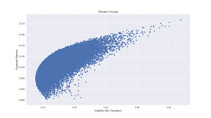
1. By doing the optimisation using Excel Solver, you are required to construct a mean variance efficient portfolio frontier for any 10 randomly selected ordinary shares listed on a stock market. For all your calculations, you should use the 60 monthly returns, sample means, standard deviations, and covariance and correlation matrices. Plot the portfolio frontier and comment on the weights of the portfolios along the portfolio frontier including in your discussion the correlations among the 10 shares.
2. Identify a risk-less asset and provide the rationale for your choice of the risk less asset.
3. By combining the risk-less asset with the 10 shares, plot the straight line efficient portfolio frontier and select the tangent portfolio on the portfolio frontier.
4. Assume that the short selling is not allowed, how your efficient frontiers would differ from those with short selling allowed in questions 1 and 3 above.
5. Identify the appropriate benchmark index and justify your choice of the benchmark index.
6. Evaluate the performance of the tangent portfolio selected above using:
a) Sharpe’s Measure
b) Treynor’s Measure
c) M2 Measure
d) Jensen’s Performance Measure
e) The Appraisal Ratio.
7. Comment on the limitation of your analysis.
8. Critically evaluate the gains in the performance of the identified portfolio along with the associated risks from investing in other asset classes, for instance, investment in gilts (including index linked), corporate bonds, convertible bonds, commodities, real estate, hedge funds and exchange traded funds.
NB
This is a portfolio optimization assignment.
It has to be done with excel after the report writing on word.
SAMPLE ANSWER
Introduction
Investing in the stock markets is highly dependent on the performance of the portfolio in which a certain investor has put his/her money. This principle of portfolio optimization was popularized by Markowitz who developed an appropriate method through which an investor could devise the most important stock portfolio for investment by avoiding risky stocks and prioritizing on investing in the stocks with the highest potential for maximum returns. Therefore, Markowitz portfolio indicates that it is necessary to increase assets and/or stocks in an investment portfolio the where the total risk of that portfolio is considered to be low or as measured by the standard deviation (or variance) of total return declines continuously, whereas the envisaged portfolio return is a weighted average of the expected returns of the individual assets. This implies that investing portfolios instead of individual assets and/or stocks, investors have a chance of significantly lowering the total risk of investing without necessarily sacrificing returns on their investments.
Therefore, the Markowitz’s mean-variance theory is usually implemented through the Excel Solver spreadsheet calculations meaning that it always optimize allocation of assets by finding the stock distribution through which there is minimization of the standard deviation or variance of the portfolio while at the same time sustaining the desired return on the stocks and/or assets. The origin of modern portfolio theory was in the 1950s with Harry Markowitz’s pioneering work in mean-variance portfolio optimization. However, prior to Markowitz’s innovation, heuristics were the ones who significantly influenced finance more than mathematical modeling. Mean-variance optimization is currently considered the core technique used by pension funds and hedge funds for portfolio diversification.
Most investors trade risk off against the envisaged return on their investments. Mean-variance optimization plays a crucial role in the identification of the investment portfolio responsible for the minimization of risk (i.e. standard deviation) for a given return. In most cases the line which is formed when the envisaged returns are plotted against the minimized standard deviation becomes the most efficient frontier for determining the most appropriate investment portfolio.
Background of Stock Portfolio Optimization
There is a certain return for every stock in the market and it is assumed that a normal distribution is portrayed by this return. This implies that the distribution for these returns for the stock can be completely described using the mean which represents the expected return as well as variance of the returns. Moreover, between any pair of stocks covariance of the returns can be computed whereby the stocks that show positive covariances, it means that they move together while the stocks that show negative covariances move in the opposite directions. Therefore, if the envisaged returns for a certain stock return or a group of stock’s returns are known, a portfolio of these stocks can be put together because of their desired variance (risk) in the stock market as a result of their envisaged return. Thus, solver, excel is mainly used for the purpose of picking the portfolio in possession of the least variance for an envisaged return meaning that the investor is likely to gain profits from his/her investment.
However, the expected return as well as the portfolio’s variance can be calculated using the method that was developed by Harry Markowitz which is crucial in the computation of portfolio return in terms of the sum of individual stock covariances and variances between stocks’ pairs in a certain portfolio. This is definitely the right thing to do from a mathematical standpoint, even though all covariances between any portfolios pair of stocks is considered meaning there would be so many calculations that would be required to accomplish this task. Alternatively, another method was devised by William Sharpe for the determination of the envisaged return and variance for a certain portfolio. This is a simpler method compared to the previous one because it assumes that any stock’s return has two parts such as the beta part which depends on the entire market performance, and the second one which is independent of the market. These two methods have been extensively used to determine the performance of specific groups of stock portfolios in the stock markets across the world for a considerable period of time.
Discussion
In our considered example, the optimal portfolio in stock market provides a risk-return trade off for superior to investing in all the shares within the UK stock exchange market. For instance, through the computations of the Excel Solver it has been determined. For instance, the portfolio optimization analysis began with the analysis of descriptive aspects of the considered 10 stock returns over a period of 60 months including means, standard deviations, and median. Moreover, the correlation and covariance matrix as well as correlation coefficient all seem to indicate that there is significant relationship between the 10 stocks considered over the 60 months.
Moreover, there are also other performance ratios such as the Treynor’s measure, Sharpe ratio, Jensen’s Performance Measure, and the appraisal ratio. For instance, Treynor’s measure of 0.4 which is relatively low considering that it is below the half mark, this implies that selected portfolio is not that better since the higher the Treynor’s measure. The Sharpe ratio is almost identical to the Treynor measure, with exception of the fact that the risk measure is the standard deviation of the portfolio rather than only considering the systematic risk, as represented by beta. Therefore, the Sharpe ratio of 1.6 is indicative of a portfolio that is not performing better. This may be attributable to the selected stock with lowly performing returns, except a few which show considerable performance.
Jensen’s Performance Measure analyses the performance of an investment by not only looking at the overall return of a portfolio, but also at the risk of that portfolio. For instance, when two mutual stocks, rationally an investor would go the one that is less risky meaning that the obtained value of 0.2 is and indicative of considerable performance of the stocks.
Finally, the Appraisal Ratio of 0.5 shows that it is necessary to attempt to beat the returns of a relevant benchmark or of the overall market. The appraisal ratio measures the portfolio performance by comparing the return of their stock picks to the specific risk of those selections, hence the higher the ratio, the better the performance of the portfolio in question.
This implies that two step must always be taken prior to determining where to invest in the stock market, where the first one regards the determination of the allocation of stocks/assets between the riskless portfolio and the risky assets and/or stocks. The second step is the determination of the allocation of resources between the risky and riskless portfolios.
However, considering that all the portfolios of riskless and risky assets have a similar Sharpe ratio, all investors do not have one optimal portfolio, but their allocation is often determined by specific factors that are individual like the objectives of the investor or risk aversion of the investor, taking into account factors like the investor’s horizon, wealth, etc. Furthermore, the extent to which the volatility of the portfolio can be decreased is highly dependent on the correlation whereby, the lower the average correlation of the stocks within a certain portfolio, then it implies that that is the lower an investor can decrease the volatility of the portfolio. This is a clear indication that this has provided the author of this assignment with succinct knowledge of determining the optimal allocations in stock markets.
Conclusion
Through this assignment it has been shown that, it is possible to use specialized spreadsheets for the calculation of important risk and return related portfolio statistics in the stock markets as well as minimizing the overall risk or maximizing the expected return of a multi-stock portfolio. However, it is essential to know that irrespective of these calculations being useful when creating investment portfolios, they rest on the assumption that historical relationships between asset classes and individual assets will hold in the future. This means that it is always crucial for investors to choose a period that they feel is representative of a “typical” market cycle, in order to avoid a capturing a repetitive cycle that is not relevant.
Moreover, the mean-variance portfolio optimization has its limitations, despite the fact that it is very helpful in choosing appropriate portfolios. For example, using standard deviation (or variance) as a proxy for risk can only be considered valid for normally distributed returns, and not any other returns which is not always the case in the stock markets. In addition, the premise of the Markowitz theory means that investors are not likely to make any alterations to their asset allocation after it has been optimized. Finally, fund managers or investors may not necessarily be interested in the minimization of risk (i.e. standard deviation or variance), but instead they may be interested in reducing the correlation of a fund to a benchmark. These are the limitations of the used method, even it is very crucial in determining portfolio optimization.
Reference List
Arnold, G. (2008), Corporate Financial Management, Third Edition, New York, NY: Pearson Education Limited.
Craig, W. H. (2008), Excel Modelling and Estimation in Investments, Third Edition, Indiana University, Prentice Hall, Inc.
FTSE Website http://www.ftse.com/products/indices/uk
Goldfarb, D. and Iyengar, G. (2003), “Robust Portfolio Selection Problems”. Mathematics of Operations Research, Vol.28 Issue 1, pp. 1-38.
Jackson, M. and Staunton, M. (2001), Advanced Modelling in Finance using Excel and VBA. Chichester, England: John Wiley & Sons.
Markowitz, H.M. (1959), Portfolio Selection: Efficient Diversification of Investments. New York, NY: John Wiley & Sons.
Markowitz, H.M. (1952). “Portfolio selection” The Journal of Finance, Vol. 7 Issue 1, pp. 77-91.
Sharpe, W.F., (1964), “Capital asset prices: A theory of market equilibrium under conditions of risk”. Journal of Finance, Vol. 19 Issue 3, pp. 425-442.
We can write this or a similar paper for you! Simply fill the order form!