Analyze the 2014 California Gubernatorial election results.
Make an educated projection for the 2018 Gubernatorial election.
This year’s election 2018 will be a midterm election. Midterm elections happen every 4 years in-between presidential election years. During these election years, we elect 1/3 of the US Senate and the US House of Representatives and state and local level public servants. During the last midterm election (2014) California voter turnout was at 42% for the November general election. Of the 24.3 million eligible California voters, 17.8 million were registered to vote in 2014. In 2010 turnout was at roughly 60% during the midterm election. California’s population has stayed at roughly 38 million people over the last 5 years. In this upcoming election 2018 we will elect a Governor of California. In the 2014 Gubernatorial election, Jerry Brown(D) secured 60% of the vote while Neel Kashkari(R) captured 40%. This years race for the Governor is between Gavin Newsom (D) and John Cox (R).
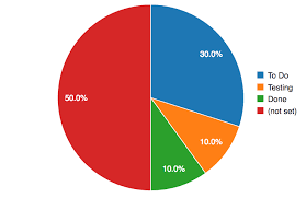
Step 1: Make a pie chart in which you show the percent of the California population that elected Governor Brown in 2014.
Step 2: Looking at the registration trends table and public opinion poll, make a prediction about this years Gubernatorial election. If you were on Newsom’s election campaign staff, what would you tell him to do? If you were on Cox’s election campaign staff what would you tell him to do?
here is an example
Step1:
In 2010
total California pop = 37.5 million
eligible voter pop = 23.5 million
Registered to vote = 17.2 million
Turned out to vote = 10.3 million or 60% of registered
Voted for Jerry Brown = 5.4 million or 53.8% of vote
Voted for Meg Whitman= 4.1 million or 40.9% of vote
Pie chart of 2014 vote
Jerry Brown was elected by 14.4% of the total population of California.
*All Data collected from the Ca Secretary of State’s Statement of the Vote
Brown has consistently polled at 40+% throughout the campaign, where Whitman has struggled at an average of 35% throughout. The poll trend line for Whitman votes leading up to the election is decreasing, meaning she is not gaining any speed but loosing traction going into the election. Based solely upon the polling results, I predict that Brown will win the election. Obviously this isn’t accounting for their difference in political experience, name recognition, gender, or other factors. If I worked on Brown’s campaign I would encourage him to campaign in the flowing light/Whitman counties with large populations: San Diego, San Bernardino, and San Los Obispo. He should also spend time in light/Brown districts such as Napa, Solano, and San Joaquin. He should particularly canvas in neighborhoods with a high density of younger voters, women, and the working class. If I was working for Whitnam I would encourage her to campaign in the same counties, while concurrently providing negative campaign adds in those counties. In addition, Whitman should try to recruit former Governor Schwarzenegger to campaign with her throughout the southern portion of the state. Given the Republican base, Whitman should particularly encourage white men and women to turnout to vote.
We can write this or a similar paper for you! Simply fill the order form!
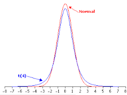
In the following situations, indicate whether you’d use the normal distribution, the t distribution, or neither.
The population is normally distributed, and you know the population standard deviation.
You don’t know the population standard deviation, and the sample size is 35.
The sample size is 22, and the population is normally distributed.
The sample size is 12, and the population is not normally distributed.
The sample size is 45, and you know the population standard deviation.
The prices of used books at a large college bookstore are normally distributed. If a sample of 23 used books from this store has a mean price of $27.50 with a standard deviation of $6.75, use Table 10.1 in your textbook to calculate the following for a 95% confidence level about the population mean. Be sure to show your work.
Degrees of freedom
The critical value of t
The margin of error
The confidence interval for a 95% confidence leve
Statistics students at a state college compiled the following two-way table from a sample of randomly selected students at their college:
Play chess Don’t play chess
Male students 25 162
Female students 19 148
Answer the following questions about the table. Be sure to show any calculations.
How many students in total were surveyed?
How many of the students surveyed play chess?
What question about the population of students at the state college would this table attempt to answer?
State Hº and Hª for the test related to this table.
Answer the following questions about an ANOVA analysis involving three samples.
In this ANOVA analysis, what are we trying to determine about the three populations they’re taken from?
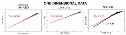
1) Choose a one-dimensional series of data, from either the dataset you described in the midterm, or from the temperature data I gave you in class.
2) Plot the whole series, using any computer plotting tool you wish.
3) Answer the question: Is it appropriate to take the variability about a mean value for this data set? The answer will be no if it includes an abrupt transition across which the behavior changes drastically. In this case you may break the series into two pieces on the sides of the transition. The answer will be no also if the data is dominated by a trend. In this case, you would need to find the trend by performing a linear fit (using linear regression or a degree-one polynomial fit) to the data, so that you can remove the trend.
4) After taking care of item 3, compute the mean, standard deviation, and find the power spectrum of the series, and/or at least two of the subseries if the set needs to be so divided. The best way of doing the power spectrum is to take the Fourier transform of the autocovariance function. (I described the autocovariance in class; there is a tool in numpy that does this that I have given you in the example I posted.) If the autocovariance is too difficult for some reason, you have permission to simply take the Fourier transform of the series; however, the spectra obtained by taking longer and longer series of data will not converge.
5) Try to identify and interpret one or more peaks in the data.
We can write this or a similar paper for you! Simply fill the order form!
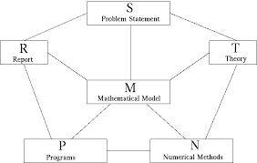
Introduction: describe system & explain question and why it is interesting
Describe model: what is being included/excluded; how do different pieces fit together; derive model/equations
[somewhere in the Introduction or Description, explain previous relevant models & why yours is different]
Describe data: what are they? from where do they come? how reliable are they?
Analyze model: explain math/computations; give results
Conclusion: what is the answer to the question, from results? discuss answer; How might model be extended/improved?
References: standard bibliographical format; citations in text; not Wikipedia.
Mathematical models are an abstract model that uses mathematical language to describe the behaviour of a system.
We can write this or a similar paper for you! Simply fill the order form!
percolation threshold xc for a wire mesh is the ratio of non-blocked sites to the total number of sites when the electrical conductance vanishes. Watson and Leath (1974) found xc=0.59 using a mesh with 18 769 nodes (137 by 137). In class we looked at a mesh with 64 nodes (8 by 8) and found a similar result.
Please follow these steps to get your own guess for site percolation threshold on the square lattice with open boundary conditions on the 64 node mesh (8 by 8)! We can then combine our guesses to get a sense of the spread of the critical regime where conductance goes to zero. Please prepare and drop-off at the beginning of class on Thursday 29 November a report with your name and student identification number at the top documenting your estimate along the following lines:
1) Take four sheets of paper and draw on each sheet a square mesh with 64 squares. For each mesh, label the rows 1,2,3,4,5,6,7,8 and the columns a,b,c,d,e,f,g,h. Each square now has a unique label such as e1, f4, and g7.
We will use the first mesh to generate a random sequence of sites to block in the second, third and fourth meshes. In the squares of the first mesh, write the label of the square. Now slice up the first mesh into its squares, put the pieces in a hat, and draw squares in order without replacing them from the hat and record the sequence you obtain. Please include the sequence in your report.
2) Now using the random sequence of labels we got in (1), mark an x in the corresponding square of the second, third and fourth meshes. As you proceed, keep track of the number of sites that you have blocked and the size of the biggest cluster of non-blocked sites, where, we say two non-blocked sites are in the same cluster if they share the same row and differ by one column or share the same column and differ by one row (in other words they are nearest-neighbors on the mesh). Please include in your report the list of sizes of the biggest cluster of non-blocked sites and a plot showing the size of the biggest cluster as a function of the number of blocked sites.
3) As you draw site labels, please record the number of blocked sites Nh when there no longer exists a cluster of non-blocked sites connecting the left edge to the right edge. Please stop adding blocked sites to the second mesh after blocking the Nh-th site, highlight the last blocked site in some way, and include this mesh with the label “Critical Percolation Cluster (Horizontal)” in your report. Similarly make a note of the number of blocked sites Nv when there no longer exists a cluster of non-blocked sites connecting the top edge and bottom edge of the mesh. Please stop adding sites the third mesh after blocking the Nv-th site, highlight the last blocked site in some way, and include this mesh with the label “Critical Percolation Cluster (Vertical)” in your report.
Please include numbers Nh and Nv in your report.
4) Please make an estimate of xc using your data: compute and include in your report xc(h)=(N-Nh)/N and xc(v)=(N-Nv)/N, where, N=8×8=64 is the number of sites in the mesh. Please include also the estimate xc(1/2)=(N-N1/2)/N, where, N1/2 is the number of blocked sites when the size of the biggest cluster of non-blocked sites is closest to thirty-two (32) or one-half of the number of sites.
We can write this or a similar paper for you! Simply fill the order form!
Summary of Articles on Geometry Sketchpad There is 3 articles and you have to write one summary about them and this is what the instructor wants.
Summary of Articles on Geometry Sketchpad
For home assignment, I attached two articles. You also have the article “Using Technology to Explore the Geometry of Navajo
Waving” that you already read (but not doing its instructions). So you have three articles to read. Now the summaries will be
different. You need to read the articles carefully and then perform suggested problems on the Geometry Sketchpad. Then you
need to include some of your own GSP constructions. Those designs that I and Mary Kay have created are there so you should not
include those that we have already created. You should do your own. Your designs could be with minor differences than ours
such as different colors and so on but should be designs that you create on GSP and transfer to your Summaries paper. This
paper, which is a summary of three papers (one is repeating one) should show that not only you read the articles but also you
could make patterns and designs using the GSP for fractals. You should send this to me by March 24 (At least 4 page formatted
including GSP illustrations).
Taylor, T., & Greenlaw, S. A. (2014). Principles of microeconomics. Retrieved from http://cnx.org/content/col11627/latest
Review Figure 7.3 (p. 161). Determine the marginal gain in output from increasing the number of barbers from 4 to 5 and from 5 to 6? Does it continue the pattern of diminishing marginal returns?
b. Compute the average total cost, average variable cost, and marginal cost of producing 60 to 72 haircuts. Draw the graph of the three curves between 60 and 72 haircuts. (Taylor & Greenlaw, 2014, p. 177)
c.The AAA Aquarium Co. sells aquariums for $20 each. Fixed costs of production are $20. The total variable costs are $20 for one aquarium, $25 for two units, $35 for three units, $50 for four units, and $80 for five units. In the form of a table, calculate total revenue, marginal revenue, total cost, and marginal cost for each output level (one to five units). What is the profit-maximizing quantity of output? (Taylor & Greenlaw, 2014, p. 203)
d. A computer company produces affordable, easy-to-use home computer systems and has fixed costs of $250. The marginal cost of producing computers is $700 for the first computer, $250 for the second, $300 for the third, and $350 for the fourth, $400 for the fifth, $450 for the sixth, and $500 for the seventh.
i. Create a table that shows the company’s output, total cost, marginal cost, average cost, variable cost, and average variable cost.
ii. At what price is the zero-profit point? At what price is the shutdown point?
iii. If the company sells the computers for $500, is it making a profit or a loss? How big is the profit or loss? Sketch a graph with AC, MC, and AVC curves to illustrate your answer and show the profit or loss.
iv. If the firm sells the computers for $300, is it making a profit or a loss? How big is the profit or loss? Sketch a graph with AC, MC, and AVC curves to illustrate your answer and show the profit or loss. (Taylor & Greenlaw, 2014, p. 204)
1. Complete the following problems:
a. Using Figure 9.2 (p. 207), suppose P0 is $10 and P1 $11. Suppose a new firm with the same LRAC curve as the incumbent tries to break into the market by selling 4,000 units of output. (Taylor & Greenlaw, 2014, p. 223).
i. Estimate from the graph what the new firm’s average cost of producing output would be.
ii. If the incumbent continues to produce 6,000 units, how much output would be supplied to the market by the two firms?
iii. Estimate what would happen to the market price as a result of the supply of both the incumbent firm and the new entrant.
1. Approximately how much profit would each firm earn?
b. Using Figure 9.6 (p. 217) draw the demand curve, marginal revenue and marginal cost curves. (Taylor & Greenlaw, 2014, p. 223).
i. Identify the quantity of output the monopoly wishes to supply and the price it will charge.
ii. Suppose demand for the monopoly’s product increases dramatically. Draw the new demand curve.
1. What happens to the marginal revenue as a result of the increase in demand?
2. What happens to the marginal cost curve?
3. Identify the new profit-maximizing quantity and price.
c. Use the following table for this problem: (Taylor & Greenlaw, 2014, p. 242).
Price Quantity TC
$25.00 0 $130
$24.00 10 $275
$23.00 20 $435
$22.50 30 $610
$22.00 40 $800
$21.60 50 $1,005
$21.20 60 $1,225
Andrea’s Day Spa began to offer a relaxing aromatherapy treatment. The firm asks you how much to charge to maximize profits. The demand curve for the treatments is given by the first two columns. The total costs are given in the third column. For each level of output, calculate total revenue, marginal revenue, average cost, and marginal cost.
i. What is the profit-maximizing level of output for the treatments and how much will the firm earn in profits?
Complete the following problems:
a. A $10,000 ten-year bond was issued at an interest rate of 6%. It is now year 9 and you are thinking about buying the bond from its owner. Interest rates are now 9%. (Taylor & Greenlaw, 2014, p. 403).
i. Would you now expect to pay more or less than $10,000 for the bond? Why?
ii. Calculate what you would be willing to pay for the bond.
b. Consider the following stock ownership situation (Taylor & Greenlaw, 2014, p. 403).
ii. What is the minimum number of investors it would take to vote to change the top management of the company?
iii. Which investors would this involve?
iv. In 1-2 paragraphs discuss if any one investor would be able to make corporate changes without the agreement of the other investors.
SAMPLE ANSWER
Math Problem
Marginal Gain in Output
Marginal gain = change in total output/change in quantity
4-5 – ([80 * 5] – [72 *4])/ (80 – 72) = 15 units per unit of labor
5-6 – ([84 *6] – [80 * 5])/ (84 – 80) = 26 units per unit of labor
The above marginal output follows the principles of diminishing marginal returns.
Average Total, Variable and Marginal Costs
Quantity
Unit Price
Fixed Cost
Total Variable costs
Total Revenue
Marginal Revenue
Total Cost (Fixed + variable)
Marginal Cost
1
$20
$20
$20
$20
–
20 + 20 = $40
–
2
$20
$20
$25
$40
20
20 + 25 = $45
$5
3
$20
$20
$35
$60
20
20 + 35 = $55
$10
4
$20
$20
$50
$80
20
20 + 50 = $70
$15
5
$20
$20
$80
$100
20
20 + 80 = $100
$30
The profit maximizing output is when; marginal cost = marginal revenue. Since there is no equilibrium in MC and MR, the closest maximizing quantity is 4.
Output and Costs
Quantity
Fixed Cost
Total Variable costs
Average Variable Cost
Total Cost (Fixed + variable)
Marginal Cost
1
$250
$450
450
$700
$700
2
$250
$700
350
$950
$250
3
$250
$1000
333.33
$1250
$300
4
$250
$1350
337.5
$1600
$350
5
$250
$1750
350
$2000
$400
6
$250
$2200
366.67
$2450
$450
7
$250
$2700
385.71
$2950
$500
ii)
The zero profit point is at the minimal point of the average curve at point c while the shutdown point is where price equals the average variable cost.
If the firm sells the computers at $300, it will be making a loss when compared to prices at $500. This is because profits at $300 will earn profits at 03cb while profits made at $500 will be 03da.
Complete the Following Problems
Figure 9.2
Selling 4,000 units of output will attract a price above p1.
II) The total amount of production supplied by the two firms would be 10,000 units.
III) The market price will be lowered since there would be more supply of goods from both firms.
b)
The monopoly firm wishes to supply its commodities at 4 units and at a price of 900.
If the demand increases, the demand curve will shift outwards.
Therefore, the marginal revenue will increase while the marginal cost curve shifts inwards. The new profit maximizing quantity and price will be where the new marginal cost curve intersects with the marginal revenue curve.
The profit maximizing level is where MC equals MR which is either arrived at by producing 40 or 50 units. Therefore, the profit at 40 units will be $80 and the profit produced at 50 units will be $75. For that reason, the firm’s maximizing profit level will be 40 units.
Complete the Following Problems
I) one would expect not to pay more for the bond since an increase in interest rates indicates an increase in the value and risk of bonds.
II) Future value = principle amount * (1 + rate) time ; 10,000 * (1 + 0.09)9 = 21, 718
Bonds i – 4.5%, n – 20 semiannual periods, interest (PMT) – 300 semiannual (6% * 10, 000 * 6/12),
Therefore, present value of the bond – 300 * [1/(1 + 0.045)20]
b) The minimum number of investors required to change the top management of a company is 3.
III) The investors would be 1, 2, and 3 who make 53% in ownership and can gather votes.
IV) Making corporate changes requires one to have more shares than the rest. This means that a shareholder who has the most number of shares can gather more votes (Taylor & Greenlaw, 2014). Therefore, one investor can make corporate changes. In this case, investor number 1 can make organizational changes without agreeing with other investors. This is because he has 20,000 shares which are 20% higher than all the rest. After all, having more shares means that one is capable of gaining more votes and has the highest ownership percentage.
References
Taylor, T., & Greenlaw, S. A. (2014). Principles of microeconomics. Retrieved from http://cnx.org/content/col11627/latest
We can write this or a similar paper for you! Simply fill the order form!
When Is the Standard Deviation Equal to Zero Order Instructions: this assignment is due on next week Wednesday, so can it be ready before next week Wednesday at 10 am, please.
When Is the Standard Deviation Equal to Zero
When Is the Standard Deviation Equal to Zero Sample Answer
The z-score shows the dispersion from the mean. It is computed using the following formula.
z-score =
Given x = 9, μ =10, and σ = 4. So,
z-score =
The population standard deviation of 0, 4, and 5 is calculated as follows:
s.d =
Thus, we need to obtain the mean =
S.d =
=
The minimum is the observation with the least value in a sample, and the maximum is the largest number. Since the observations 1, 1, 2, 3, 5, 8, 13, 21, 34, 55, 89, 144, 233 are arranged in ascending order, the first observation is the minimum and the last maximum.
Minimum = 1
Maximum = 233
To obtain the first quarter (25%) we multiply the number of observations (n = 13) by 25%.
= =0.25*13 = 3.25
Thus, the 4th observation is the first quarter.
First quarter = 3
The median is the observation at the center/middle (13/2 = 6.5 = 7th observation)
Inter-quartile range =upper quartile – lower quartile
= 89 – 3
= 86
A standard deviation of zero deduces that the data sample are not spread, which in other words means that they are clumped around a single value (Taylor, 2015).
It is expected that about 95% of the observations to lie between 2 standard deviations of the mean.
It is anticipated that about 98.8% of the observations to lie between 2.5 standard deviations of the average.
Normally distributed means that the population distribution has a bell-shaped density curve, which can be described by its mean (average) and standard deviation. Furthermore, the density curve is symmetrical, clustered around the mean, and the standard deviation determines the spread of the plot.
P (x < 60000) = z () =
P (x < 60000) = 0.8413
Therefore, 84.13% of people have salaries of $60,000or less.
P (x < 40000) = z () =
=
=
= 0.1587
Therefore, 15.87% of people have salaries of $40,000or less.
When Is the Standard Deviation Equal to Zero References
Taylor, C. (2015). When Is the Standard Deviation Equal to Zero? Retrieved July 16, 2016, from http://statistics.about.com/od/Mathstat/fl/When-Is-the-Standard-Deviation-Equal-to-Zero.htm
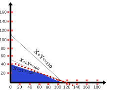
Just need to finish 4 simple question of linear programming of max/min problem.
you need to use excel (solver) in order to finish this.
ps i need to send you the question and some of the tut which similar to the assignment.
SAMPLE ANSWER
QUESTION 1
Let:
X1 = number of large aircrafts
X2 = number of medium aircrafts
X3 = number of small aircrafts
Max z: 8×1 + 5×2 + 2×3
Purchasing LP model: 8×1 + 5×2 + 2×3 120
Number of aircrafts serviced
Capacity of aircrafts in tone-miles
Fixed operating costs:
The Excel solver screenshot:
QUESTION 2
Max:
St.LP with optimal solutions
Value of objective function
QUESTION 3
Let x1 = Number of beds to produce
And x2 = Number of desks to produce
The LP model for the problem is:
Max z: 30x1 + 40x2
Subject to: 6x1 + 4x2 36
4x1 + 8x2 40
x1, x2 0
QUESTION 4
Because values of zero (0) in the “Allowable Increase” or “Allowable Decrease” columns for the Changing Cells indicate that an alternate optimal solution exists.
Initial R.H.S. = 15
Increased R.H.S. = 20
Allowable Increase = 45
This mainly because increasing the RHS value would definitely lead to increased optimal function value within the feasible region on basis of the allowable increase value provided.
25.
Initial R.H.S. = 15
Decreased R.H.S. = 12
Allowable Decrease = 5
This mainly because decreasing the RHS value would definitely lead to decreased optimal function value within the feasible region on basis of the allowable decrease value provided.
Initial R.H.S. = 20
Increased R.H.S. = 32
Allowable Increase = 10
This mainly because increasing the RHS value would definitely lead to increased optimal function value within the feasible region on basis of the allowable increase value provided.
This is due to the fact that there would be an reduction in resources utilization leading to increased productivity.
x1
const 1
const 2
0
8
5
1
6
4
2
4
3
3
1
1
References
Anderson D., Sweeney D., & Williams T (2007). An Introduction to Management Science. London: West Publisher.
Arsham H. (2007). An Artificial-Free Simplex Algorithm for General LP Models, Mathematical and Computer Modelling, 25(1), 107-123.
Arsham H. (2012). Foundation of Linear Programming: A Managerial Perspective from Solving System of Inequalities to Software Implementation, International Journal of Strategic Decision Sciences, 3(3), 40-60.
Chvatal, V. (2013). Linear Programming. New York, NY: W. H. Freeman and Company.
Lawrence J., Jr., & Pasternack, B. (2012). Applied Management Science: Modeling, Spreadsheet Analysis, and Communication for Decision Making. Hoboken, NJ: John Wiley and Sons.
Roos C., Terlaky, T. & Vial, J. (2009). Theory and Algorithms for Linear Optimization: An Interior Point Approach. Hoboken, NJ: John Wiley & Sons.
Shenoy G.V. (2010). Linear Programming: Methods and Applications. Hoboken, NJ: John Wiley & Sons.
We can write this or a similar paper for you! Simply fill the order form!
Can you please write the answers on the white paper, scan it and send me.
Thanks,
Customer.
SAMPLE ANSWER Question 14
A1 S>0, 5×7-62 = -1,
So, not positive definite
A2 -1<0, so not positive definite.
A3 1>1, 1×100-10×10 = 0,
So, not positive definite
A4 1>, 1×101-10×10 = 1
So, it is positive definite
If x1 = 1, x2=-1, then this product is 0.
Question 18
Solutions:
K=ATA is symmetric positive definite if and only if A has independent columns
For, columns of A are independent. So ATA will be positive definite.
For, columns of A are independent. So ATA will be positive definite.
For, columns of A are independent. So ATA will not be positive definite.
Question 7
Since a matrix is positive-definite if and only if all its eigenvalues are positive, and since the eigenvalues of A−1 are simply the inverses of the, eigenvalues of A, A−1 is also positive definite (the inverse of a positive number is positive).
Question 14
Positive
Negative definite
Indefinite
Negative definite
Question 15
False
False
True
True
Question 32
Question 41
On the one hand, Ax =λMx is the same as CTACy =λy (writing M = RTR for C = R−1, and putting Rx = y). Then yTBy/yTy has its minimum value at λ1(B=CTAC), the least eigenvalue for the generalized eigenvector problem. On the other hand, this quotient is equal to xTAx/xTMx, which sometimes equals a 11/m11, e.g., when x equals the standard unit vector e1.
Problem Set 6.3
Question 2
Question 5
As ?=0 corresponds with , does not enter the picture
References
Bretscher, O. (2004). Linear Algebra with Applications, (3rd ed.). New York, NY: Prentice Hall.
Farin, G., & Hansford, D. (2004). Practical Linear Algebra: A Geometry Toolbox. London: AK Peters.
Friedberg, S. H., Insel, A. J., & Spence, L. E. (2002). Linear Algebra, (4th ed.). New York, NY: Prentice Hall.
Leon, S. J. (2006). Linear Algebra with Applications, (7th ed.). New York, NY: Pearson Prentice Hall.
McMahon, D. (2005). Linear Algebra Demystified. New York, NY: McGraw–Hill Professional.
Zhang, F. (2009). Linear Algebra: Challenging Problems for Students. Baltimore, MA: The Johns Hopkins University Press.
We can write this or a similar paper for you! Simply fill the order form!