Please Answer the question respectively, each question page.
Q1 TIP/LEARNING: Think about why you move. Do you participate for skill or knowledge?
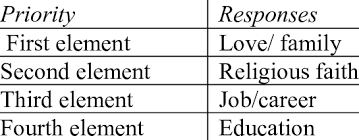
Meaning is individual. Rank why you do physical activity. Is it for Skill, Fitness, Knowledge, or Pleasure? Even though you
may do movement for prudential reasons, a better way to view movement is through skill and pleasure. Skill and pleasure should
be ranked above fitness and knowledge on their capacity to help experience the good life.
Propositions about significant living are not difficult to locate. The Bible, the Koran, scriptures, hundreds of sages of wise
people, and thousands of pop psychology and philosophy books can supply them…The fact is that we grow into stories and meaning
more than we encounter them as foreign propositions or theories. Cultural traditions, hobbies, dances, games, habits, crafts
and other activities point us in some directions and away from others. The skills we learn tell us implicitly that it is
important to do this and not that. Moreover, these activities come loaded with values—with etiquette, with ways of behaving,
with right attitudes and so on. By learning play and game skills, we grow into rights and wrongs, values and disvalues, things
that are important and other things that are not valuable…Games and play resonate with the dominant messages of our time and
place, and this builds a compass into our being that tells us the directions in which we should develop our personal stories.
(Kretchmar, R.S., (1993). Practical Philosophy of Sport, p.167)
**CHALLENGE: Try adding a(nother) fruit or vegetable serving to your daily food intake.
Reflection:
In what ways does your activity class contribute to your skill development? What do you participate in that contributes to
your skill development?
Q2TIP/LEARNING: What is the purpose of exercise? The purpose should be about helping develop and maintain a good life.
The Good Life refers to an overall life condition and set of experiences that we regard as desirable. While most everybody
aims at good living, there is considerable disagreement about what exactly it is. There are probably hundreds of ways to
achieve something called the good life, and there are undoubtedly many patterns that are comparably good. (Kretchmar, R.S.,
(1993). Practical Philosophy of Sport, p.111)
The good life is composed of experiences that are appreciated for their own sake. The good life must be meaningful or have
purpose. One event must be meaningful or have purpose. One event must be connected to another, and these events must be headed
somewhere important as in the development of a story line. Survival and long life, by themselves do little to assure good
living.
A good life should entail pleasure and fun, which is almost universal. Movement should bring meaning to your life. The good
life should be meaningful, and physical activity should bring meaning. (Kretchmar, R.S., (1993). Practical Philosophy of
Sport, p.224)
Reflection:
We can write this or a similar paper for you! Simply fill the order form!
The writer will have to read each of this post and react to them by commenting, analyzing and supporting with relevant articles. The writer will have to read carefully before giving constructive comments on the post. The writer should write a one paragraph of at least 150 words. APA and in text citation must be use as each respond to the two post must have in text citations. The writer will have to use an article to supports his comments in each of the article. Address the content of each post below in a one paragraph each, analysis and evaluation of the topic, as well as the integration of relevant resources.
It is important that the writer avoid grammatical errors and use constructive feedback in the two articles.
I will send the articles via email
SAMPLE ANSWER
In dataset 1. Most of the analysis performed were sufficient for the purpose of the inferential statistics. This is because the p-value was used in making inference about the sample data (Ireland, 2010). Nevertheless, the tables were not formatted by APA 6th edition guideline (Szuchman, 2013). The writer opts to modify the table looks such that their appearance resembles that of an APA table format. Furthermore, some of the in-text citation did not follow the APA guideline. Furthermore, the inference made was incorrect; the hypothesis is never accepted, it is just lack of adequate evidence that leads to failing to reject. Thus, the inference was supposed to state: we fail to reject the null hypothesis due to lack of enough evidence (Ireland, 2010). Furthermore, the hypothesis should be restructured to look more professional, and on the same note the null hypothesis are denoted by (H0 or Ha), and the alternative hypothesis with (H1 or Hb) (Masson, 2011).
In data set 2: the APA file formatting is well observed in the table formatting (Szuchman, 2013). Furthermore, the research paper is well written, since the writer wrote the research question that will act as a blueprint for his/her analysis. Nevertheless, the descriptive statistics were supposed to give the distribution of data, which is the spread of data (Ireland, 2010). On the same note, the writer cannot make an inference based on the descriptive statistics, which are used to construct the confidence interval. Thus, logical analysis like ANOVA analysis ought to have been carried out to measure the variability of the variables (Hecke, 2012). These tests are powerful, and they are used in the inferential statistics. In particular, to test whether there exists statistical difference between variables. Similarly, the writer should not say that the null hypothesis is accepted (fail to reject) (Masson, 2011).
Ireland, C. (2010). Inferential statistics and hypothesis testing. Experimental statistics for agriculture and horticulture, 62-70.
Masson, M. E. (2011). A tutorial on a practical Bayesian alternative to null-hypothesis significance testing. Behavior research methods, 43(3), 679-690.
Szuchman, L. (2013). Writing with style: APA style made easy. Cengage Learning.
We can write this or a similar paper for you! Simply fill the order form!
Data Interpretation Practicum using SPSS Software Order Instructions: Your Data Interpretation Practicum
Data Interpretation Practicum using SPSS Software
Throughout the course, you will learn to run various statistical analyses using SPSS (PASW) software. Part of your work will include analysis and interpretation as well. In addition, doctoral-level thinking and practice involve the formation of hypotheses, their testing, working with data, and the selection and execution of appropriate analyses. Toward that end, your Instructor will expect you to demonstrate your ability to engage in these doctoral-level competencies as you progress through the course.
A series of incremental Applications will allow you to demonstrate your accrued competency. This week, you will select the dataset from which you will work in subsequent weeks. Having learned to perform various analyses in SPSS (PASW), you will then perform them on your chosen data in subsequent weeks, interpreting the results and presenting them in accordance with APA conventions.
Use the attached dataset and respond to the following. Explain how it relates to your interests (EFFECTS OF HRM PRACTICES ON EMPLOYEE PERFORMANCE), what hypotheses might you test? What would you expect to find? At this point, an educated guess and a general idea are sufficient. However, your submission should demonstrate that you have examined the data and that you understand what it comprises. Be sure to include the name of the database as well as 1–2 paragraphs that address these questions.
Data Interpretation Practicum using SPSS Software Sample Answer
Introduction
Thepurpose and objective of this paper are to analyse the ‘Data for week one assignment’. This research will establish whether there exists any relationship between the rate of injuries in a working site with the gender of supervisor managing the site, the number of employees at the site, and a number of hours the employees are working.This isa great research problem for research on since it is related to the practice of human resource management on the employee’s performance. In particular, it will establish whether an individual supervisor’s gender contributes to the high injury rate in a site, increase the number of employees increases the injury rate and also if the increased number of working hours is positively correlated to the injury rate.
In light of this, the provided data will be analyzed using SPSS for windows and inference given about the population. The basis of the analysis will be to infer about the following hypothesis:
H0: There is no significance difference in injury rate at a working site and supervisor’s gender, number of employees and the number of hours at work.
H1: There is a significance difference in injury rate at a workingsite and supervisor’s gender, number of employees and the number of hours at work.
The stated hypothesis leads to the formulation of the following research question: Is there a significance difference in injury rate at a workingsite and supervisor’s gender, number of employees or the number of hours at work. Thus, the primary task carried out in data analysis will be to infer about the population using the sample data given at the 95 % level of significance.
Analysis
In search of answering the research question, a one-way ANOVA was performed. This was an appropriate measure since it measures the variability of data relative to the mean of the variables. In this case, the injury rate was considered as the factor (dependent variable) (Murphy, 2014). The results of the off the analysis are summarized in Table 1.
Table 1:
ANOVAresults summary
Sum of Squares
df
Mean Square
F
Sig.
number of employees
Between Groups
2263.147
33
68.580
2.136
.050
Within Groups
545.833
17
32.108
Total
2808.980
50
supervisors gender
Between Groups
7.973
33
.242
.868
.648
Within Groups
4.733
17
.278
Total
12.706
50
number of hours at work
Between Groups
9791279435.294
33
296705437.433
2.136
.050
Within Groups
2361493333.333
17
138911372.549
Total
12152772768.627
50
The decision here is to reject the null hypothesis when |F calculated| > F tabulated. The F 0.05, (33, 17) = 2.15, at critical value (α = 0.05). Since the F calculated values ofnumber of employees, hours worked, supervisors gender are less than 2.15 we fail to reject the null hypothesis that they have no significance difference. In fact, we state that they show no significant difference at the 95% level of significance(Ashton, 2013). In other words, there is no significant difference in injury rate at a working site and supervisor’s gender, number of employees and the number of hours at work.
To test the nature of the association between this variable. A correlation analysis was performed in agreement with (Wilcox, 2012). The results are as tabulated in Table 2.
Table2:
Correlations coefficient summary
injury rate
number of employees
supervisors gender
number of hours at work
injury rate
Pearson Correlation
1
-.636**
-.090
-.636**
Sig. (2-tailed)
.000
.532
.000
N
51
51
51
51
number of employees
Pearson Correlation
-.636**
1
.236
1.000**
Sig. (2-tailed)
.000
.096
.000
N
51
51
51
51
supervisors gender
Pearson Correlation
-.090
.236
1
.236
Sig. (2-tailed)
.532
.096
.096
N
51
51
51
51
number of hours at work
Pearson Correlation
-.636**
1.000**
.236
1
Sig. (2-tailed)
.000
.000
.096
N
51
51
51
51
**. Correlation is significant at the 0.01 level (2-tailed).
The Pearson’s correlation coefficient indicate that the association between the injury rate with the number of employees, and number of hours at work is negative(Lowry, 2014). In particular, the number injury rates reduceas the number of workers and number of working hours increases. Nevertheless, supervisor gender has a weak negative association with injury rate.
From the analysis, it is clear that the research objectives have been achieved and also the hypothesis has been taken care. In this study, there was no adequate evidence to reject the null hypothesis thus the inference that will hold is there is no significance difference in injury rate at a workingsite and supervisor’s gender, number of employees and the number of hours at work.
Data Interpretation Practicum using SPSS Software References
Wilcox, R. R. (2012). Introduction to robust estimation and hypothesis testing. Academic Press.
Ashton, J. C. (2013). Experimental power comes from powerful theories [mdash] the real problem in null hypothesis testing. Nature Reviews Neuroscience,14(8), 585-585.
Lowry, R. (2014). Concepts and applications of inferential statistics.
Murphy, K. R., Myors, B., &Wolach, A. (2014). Statistical power analysis: A simple and general model for traditional and modern hypothesis tests.Routledge.
This paper will be a continues paper and the writer must have a very good understanding of using the software mentioned in this paper. It is critical that the writer stay consistent with all of this paper most importantly reading all instructions and properly following directions to complete each section of the paper. This particular paper consist of 3 main parts to complete and the writer must clearly respond to this 3 main points listed in APA 6th edition. I will email the main dataset mentioned in the questions which will enable the writer to complete this paper. The writer must thoroughly analyze the data as require using the proper means.
For this assignment you use SPSS (PASW) software and learn to properly manipulate data according the APA requirements. This is an important skill and will be a major factor in future assignments in this course, your doctoral studies and dissertation. It is strongly encouraged that you review Chapter 5 of the APA Publication Manual to understand table and figure requirements before starting.
Follow the directions for using SPSS (PASW) in this assignment:
You will then write a 3-4 page paper in which you present your table and an analysis of your findings. Keep in mind that you cannot draw conclusions without further testing. Instead identify notable trends, patterns, relationships, associations, etc. Your paper must meet the following requirements:
• Include an opening including thesis statement, body and conclusion.
• Include a properly stated research question
• Include a properly formatted null and alternative hypotheses
• Follow APA (American Psychological Association) style and include in-text citations and a separate references page
• Software
• IBM SPSS Statistics Standard GradPack (current version). Available in Windows and Macintosh versions.
Course Text(s)
• Green, S. B., & Salkind, N. J. (2014). Using SPSS for Windows and Macintosh: Analyzing and understanding data (7th ed.). Upper Saddle River, NJ: Pearson.
o Units 1 and 2, pp. 1–50
? Lesson 1, “Starting SPSS”
? Lesson 2, “The SPSS Main Menus and Toolbar”
? Lesson 3, “Using SPSS Help”
? Lesson 4, “A Brief SPSS Tour”
? Lesson 5, “Defining Variables”
? Lesson 6, “Entering and Editing Data”
? Lesson 7, “Inserting and Deleting Cases and Variables”
? Lesson 8, “Selecting, Copying, Cutting, and Pasting Data”
? Lesson 9, “Printing and Exiting an SPSS Data File”
? Lesson 10, “Exporting and Importing SPSS Data”
? Lesson 11, “Validating SPSS Data”
This text includes a series of step-by-step tutorials for using SPSS statistical software to enter data; generate statistics, charts, and graphs; and format SPSS output in APA style. Tutorials include screenshots as well as real-world examples of the statistics in question.
Datasets
• Pearson Education. (2010). Datasets to accompany Using SPSS for Windows and Macintosh by Green and Salkind [Data file]. Retrieved from http://www.prenhall.com/greensalkind/GreenSalkind.zip copy and paste to retrieve.
Please Note: The SPSS maximum variable data length is 1,500 variables.
Note: You will need a file-compression program, such as WinZip, to unzip this file.
• Main Dataset
Articles
• Corner, P. D. (2002). An integrative model for teaching quantitative research design. Journal of Management Education, 26(6), 671–6 92.
Retrieved from ABI/INFORM Global database.
This article highlights the quantitative research reasoning and process that typifies the stages in a quantitative study. It likens each stage—f ormulating a problem statement, crafting a hypothesis, collecting data, analyzing data, and interpreting findings—to a corresponding step in its proposed integrative model.
Readings
• American Psychological Association. (2010). Publication manual of the American Psychological Association (6th ed.). Washington: Author.
This text is the preferred style manual for business researchers and provides guidance on the formatting and presentation of research conducted with statistical software.
This text teaches the beginning statistician when and how to apply different statistical tests. Written as a resource for those without an extensive statistical background, it includes descriptions, illustrations, and solved examples.
Note: The link above takes you to a preview version of the chapter from the publisher and only includes samples of the pages rather than the full text. Click on the “Next” and “Previous” buttons in the upper right of the page to navigate the chapter.
Websites
• Trochim, W. (2006). Web center for social research methods: Selecting statistics. Retrieved from http://www.socialresearchmethods.net/
This site is an online textbook that addresses the topics of a typical graduate course in social research methods, including sampling, measurement, validity, types of designs, and analysis. Learners can navigate the textbook using a graphical research road map or simple table of contents. The textbook addresses the entire research process as well as the statistical aspects of research and is not software-specific. From the main page, click on the ” Selecting Statistics” link.
SAMPLE ANSWER
Introduction
The main purpose of this paper is to analyze the dataset aiming to establish trends, patterns relationship, and association and establishing whether there exists a relationship between different variables. Thus, the basis of this paper will be to understand the raw data after analysis (Kraemer, 2015). The output of the analysis will help in noticing different spread and distribution of data. To achieve this SPSS for Windows software will be used to analyze the data provided, notably all the tables and figures will be formatted in American Psychological Association (APA) formatting style. Through this, a masterpiece work will be achieved and some inference drawn about the sample population.
The research will be guided by the following research question: is there a significant difference in injury rate at different working sites when different genders are managing or at a different risk factor?
The stated research questions will act a blueprint and foundation for all analysis that will be carried out (Kraemer, 2015). The research will be based on the hypothesis:
H0: there is no significance difference in injury rate at different working sites when different genders are managing or at different risk factor.
H1: there is a significance difference in injury rate at different working sites when different genders are managing or at different risk factor.
Thus, the purpose of this paper is to make an inference reject or fail to reject the set claim. To achieve this, a number of analyses will be carried out at 95% level of significance.
Data analysis
The following tables show the frequency distribution of sites, the gender of the supervisors, and risk factor.
Table 1: Site frequency distribution
Frequency
Percent
Valid Percent
Cumulative Percent
Valid
Boston
15
29.4
29.4
29.4
Phoenix
19
37.3
37.3
66.7
Seattle
17
33.3
33.3
100.0
Total
51
100.0
100.0
Table 2: SupervisorGender frequency distribution
Frequency
Percent
Valid Percent
Cumulative Percent
Valid
Female
27
52.9
52.9
52.9
Male
24
47.1
47.1
100.0
Total
51
100.0
100.0
Table 1 shows that most of the supervisors involved in the research come from Phoenix with a 37.3%, followed by 33.3% from Seattle, and Boston had the least supervisors in the sample. Also, the sample consists 52.9% females and 47.1% males, which is illustrated in Table 2.
To answer the research question whether there exists a relationship between genders of the supervisor, the number of employees, the number of working hours, a risk factor with injury rate, a one-way ANOVA was performed (Gelman, 2014). The results are shown in Table 4.
Table 4: ANOVA table summary.
Sum of Squares
df
Mean Square
F
Sig.
NumEmps
Between Groups
2263.147
33
68.580
2.136
.050
Within Groups
545.833
17
32.108
Total
2808.980
50
Hours_Worked
Between Groups
9791279435.294
33
296705437.433
2.136
.050
Within Groups
2361493333.333
17
138911372.549
Total
12152772768.627
50
SupervisorGender
Between Groups
7.973
33
.242
.868
.648
Within Groups
4.733
17
.278
Total
12.706
50
Risk
Between Groups
168.286
33
5.100
2.545
.022
Within Groups
34.067
17
2.004
Total
202.353
50
The decision here is to reject the null hypothesis when sig. < The critical value (α = 0.05). Since the sig. Value of number of employees, hours worked, supervisors gender are greater or equal to 0.05 we fail to reject the null hypothesis that they have no significance difference (Andraszewicz, 2014). In that matter, we conclude that they show no significant difference at the 95% level of significance. Nevertheless, risk factor shows significance difference since its p-value is less than the critical level.
To measure the nature of the association between these factors with injury rate, a correlation analysis was done on the data set. The results obtained were as follows.
Table 5: Correlations
number of employees
number of hours at work
injury rate
supervisors gender
risk factor
site
number of employees
Pearson Correlation
1
1.000**
-.636**
.236
.351*
.130
Sig. (2-tailed)
.000
.000
.096
.012
.363
N
51
51
51
51
51
51
number of hours at work
Pearson Correlation
1.000**
1
-.636**
.236
.351*
.130
Sig. (2-tailed)
.000
.000
.096
.012
.363
N
51
51
51
51
51
51
injury rate
Pearson Correlation
-.636**
-.636**
1
-.090
-.433**
-.074
Sig. (2-tailed)
.000
.000
.532
.001
.606
N
51
51
51
51
51
51
supervisors gender
Pearson Correlation
.236
.236
-.090
1
.096
-.047
Sig. (2-tailed)
.096
.096
.532
.501
.745
N
51
51
51
51
51
51
risk factor
Pearson Correlation
.351*
.351*
-.433**
.096
1
.272
Sig. (2-tailed)
.012
.012
.001
.501
.054
N
51
51
51
51
51
51
Site
Pearson Correlation
.130
.130
-.074
-.047
.272
1
Sig. (2-tailed)
.363
.363
.606
.745
.054
N
51
51
51
51
51
51
**. Correlation is significant at the 0.01 level (2-tailed).
*. Correlation is significant at the 0.05 level (2-tailed).
As illustrated, there exists a moderate negative correlation between injury rate and risk, number of employees, and number of working hours (Murphy, 2014). However, a weak negative correlation of -0.090) between injury rate and gender of supervisor exists and -0.073986 between injury rate and site (Andraszewicz, 2014).
A model that can predict injury rate using risk, supervisor gender, hours worked, and site as the predictors in the model was as follows;
Injury rate = 53.053735 + 2.559949*(supervisor gender) – 0.000642 * (hours worked) – 2.256611 * (risk) + 1.628766*(site). Nevertheless, the F-table that was obtained after the regression analysis is as tabulated below.
Table 6: ANOVAa
Model
Sum of Squares
df
Mean Square
F
Sig.
1
Regression
7093.819
4
1773.455
9.980
.000b
Residual
8174.037
46
177.696
Total
15267.856
50
a. Dependent Variable: InjuryRate
b. Predictors: (Constant), Site, SupervisorGender, Hours_Worked, Risk
The decision rule is to reject the null hypothesis when |F calculated|> F tabulated. In this case, F calculated = 9.980 > F 0.05 (3, 47) = 2.61, thus we reject the null hypothesis (Kass, 2014). This means in agreement with (Kraemer, 2015) that there exists a significant difference between these variables.
Conclusion
To sum up all, the primary objective of the research has been achieved, since an inference has been made about the sample population. The analysis has led to the rejection of the null hypothesis, thus concluding that there is a significance difference in injury rate at different working sites, when different genders are managing or at different risk factor. Hence, in a comprehensive way the questions that were posed at the beginning have been fully answered.
References
Kass, R. E., Eden, U. T., & Brown, E. N. (2014). Analysis of Variance. In Analysis of Neural Data (pp. 361-389). Springer New York.
Kraemer, H. C., & Blasey, C. (2015). How many subjects?: Statistical power analysis in research. Sage Publications.
Andraszewicz, S., Scheibehenne, B., Rieskamp, J., Grasman, R., Verhagen, J., & Wagenmakers, E. J. (2014). An introduction to Bayesian hypothesis testing for management research. Journal of Management, 0149206314560412.
Murphy, K. R., Myors, B., & Wolach, A. (2014). Statistical power analysis: A simple and general model for traditional and modern hypothesis tests. Routledge.
Gelman, A., Carlin, J. B., Stern, H. S., & Rubin, D. B. (2014). Bayesian data analysis (Vol. 2). London: Chapman & Hall/CRC.
We can write this or a similar paper for you! Simply fill the order form!
For this assignment you write a paper covering answers to assigned problems in Lessons 22 and 23 of your course text.
Lesson 22: problems 1–4 (page 150)
Lesson 23: problems 1–5 (page 155)
Your paper should be written using APA 6th edition guidelines. There is a sample paper on page 41 of the Publication Manual which you may use as a reference.
Your paper must meet the following requirements:
Include explanation and justification of all answers. (Answers to some questions can be found in back of text to use as frame of reference)
Include an APA Results section for each problem set. (There is an example on page 167 of the course text)
Include presentation, discussion and explanation of all figures and tables
Include only the critical elements of your SPSS output
Include a properly formatted H10 (null) and H1a (alternate) hypothesis which cover all possible situations related to a problem
Include an examination of statistical testing to the null using the statement “fail to reject” or “accept”. (Notice the language is always related to the null hypothesis)
Include not only the results of the testing, but the steps you took to conduct the test via SPSS.
Additionally, you must provide a table to demonstrate that portion of the assignment
SAMPLE ANSWER
Annotated bibliography
Galliers, R., & Currie, W. (2011).The Oxford Handbook of Management Information Systems. Oxford: OUP Oxford.
Scope-Management Information Systems play a crucial role in the accounting, operations, decision-making, competitive advantage, and organization’s operations. The Oxford Handbook of Management Information Systems discusses in broad the increasing complexity of the systems in relation to strategic, managerial, organizational and managerial issues. The book is classified into four broad categories i.e. the background to the topic, theoretical and methodology in use, issues to do with ethics and rethinking MIS in a broader way.
Purpose and methodology-The purpose of the book is the discussion of the increasing complexity in MIS. It employs a multi-disciplinary approach in the discussion of MIS.
Underlying assumptions-It assumes that no individual has a perfect knowledge about the future trends when it comes to issues to do with MIS. The book however offers a vivid explanation about the MIS scenario enabling the reader to understand all the concepts with ease.
The limitation is that, it does not offer the reader an opportunity to get practical examples in MIS as most of the coverage is theoretical. Opportunities for further learning are present as the learner understands how the future facets will shape the accounting process.
Jinnette, J. (2010). The relevance of intangible assets in the context of the managerial accounting decision making process.
Scope-The book offers an in-depth analysis of how intangible assets affect the MIS process. It assumes that every organization has two sets of assets i.e. the tangible assets and the intangible assets. The book broadly discusses how the various intangible assets need to be treated in the control and planning process. The research process provided the relevant data in the writing of the book.
The limitation is that it does not give the relationship that exists between the accounting of the intangible assets and the other facets of the organization such as the human resource. Individual understanding is that, the facets are interrelated.
.Libby, R., Libby, P., & Short, D. (2011).Financial accounting. New York: McGraw-Hill/Irwin.
Scope-the financial position is related with the working of MIS. The book set out to explain the relationship that exists between financial accounting and Managerial accounting. The approach that the book use is research across the existing research works. A considerable amount of data gathered led to the publication of the book. The key assumption is that, financial accounting is a feeder program of managerial accounting. It therefore acts as the main control agent in accounting.
Compared to other sources evidenced earlier, it is more detailed in providing the comparison between financial accounting and managerial accounting. The limitation is that, it does not address how the changing cases in the field of finance will affect the accounting process. Further studies can be conducted in the analysis of the various cost items in the accounting process.
Mancini, D., Vaassen, E., &Dameri, R. (2013).Accounting information systems for decision making. Berlin: Springer.
The book clearly details how accounting information available to the management will shape up the process of decision making. The purpose of the book that was written entirely through research is to smoothen decision making by getting accounts right as well as aligning the management. The key assumption is that, for perfect decisions to be made there is perfect information flow. The limitation is that, the systems discussed are not well situated for the rapid changes occurring in the management sector. Studies can be done in the are to align the existing systems so that they are well suited for future action.
Lambert, R. (2012).Financial literacy for managers. New York: Wharton Digital Press.
The managers are given detailed information on how to run the organization in a convenient manner by observing a clear rule of not spending beyond their means.It offers managers the key lessons on effective finance management. It was also written through research. It assumes that an organization is controlled by a set of both internal and external factors. It has no control over its’ external factors but it can control the internal factors, finance being one of them. It is important as it sheds light on the methods through which financial literacy can enhance decision making.
McNair, C. (2013). Value creation in management accounting. New York: Business Expert Press.
The control process is discussed as a means by which the management needs to produce a certain value within the whole organization. It places on emphasize on value creation among managers. Research enabled the writing of the book. The assumption is that, value created by financial factors is not entirely by the management, the management need to combine a set of both innovative and solution seeking means.
Lu, J., Jain, L., & Zhang, G. (2012).Handbook on decision making. Heidelberg: Springer.
The book provides managers with the key guidelines in making their day to decisions within the organization. It provides an enabling environment to the management for effective decision making. The book was entirely written through research. The assumption is that, an organization uses the top-down approach in decision making.
Libby, R., Libby, P., & Short, D. (2011).Financial accounting. New York: McGraw-Hill/Irwin.
Finance is one of the key concepts that are necessary for effective control of the organization. The need for managers to understand financial accounting, so that they can handle matters to do with control is well covered by the book. Research by the writers was the methodology that enabled writing of the book. The key assumption is that, financial accounting is a feeder program of managerial accounting. It therefore acts as the main control agent in accounting.
Compared to other sources evidenced earlier, it is more detailed in providing the comparison between financial accounting and managerial accounting. The limitation is that, it does not address how the changing cases in the field of finance will affect the accounting process. Further studies can be conducted in the analysis of the various cost items in the accounting process.
Afzal, W. (2012).Management of information organizations. Oxford, UK: Chandos Pub.
The book places emphasize on the importance of managers getting the information concept within the organization right. Managers are given effective information on how to manage information within the organization during the control process. The research process enabled the writers to write the book. The assumption is that, information within an organization can assume both the vertical and horizontal means of flow.
Pham, K. (2012). Linear-Quadratic Controls in Risk-Averse Decision Making. New York: Springer.
The book majorly centers on the importance managers derive by keenly analyzing the decisions they make under a risky situation.The book articulates for the importance of individuals not being risk averse in the process of decision making. Research was essential in the process of writing the book. The assumption is that, risky situations are not admired by most of the decision makers. It offers important lessons on why managers need to be risk takers for effective decision making. Further analysis can be done in aligning the current state in line with the future prospects which are usually risky.
We can write this or a similar paper for you! Simply fill the order form!
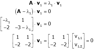
The matrix has eigenvalues1=3 and 2=−2. Let’s find the eigenvectors corresponding to 1=3. Let v=v2v1. Then(A−3I)v=0 gives us
2−3−1−4−1−3v1v2=00 from which we obtain the duplicate equations
−v1−4v2−v1−4v2=0
If we let v2=t, thenv1=−4t. All eigenvectors corresponding to1=3are multiples of1−4 and thus the eigenspace corresponding to1=3is given by the span of1−4. That is,1−4is a basis of the eigenspace corresponding to 1=3.
Repeating this process with 2=−2, we find that
4v1−4V2−v1+v2=0
If we let v2=t then v1=t as well. Thus, an eigenvector corresponding to2=−2 is 11 and the eigenspace corresponding to 2=−2 is given by the span of11. 11is a basis for the eigenspace corresponding to 2=−2.
Problem 3
Problem 5
Problem 14
Problem 22
Problem 25
Matrices A2 and A3 cannot be diagonized because for a square matrix A, wherever A is similar to diagonal matrix then the matrix is diagonizable.
Problem 15-24: Eigenvalues & Eigenvectors Matrices
Problem 15
Since all entries are ≥ 0 and each column sums to 1, this A is a Markov matrix. Thus we know that λ1 = 1 is an eigenvalue. Since tr(A) = λ1 + λ2 = 3/2, we conclude λ2 = 1/2 is another eigenvalue. We diagonalize it using the matrix S of eigenvectors:
= → =
This last matrix product equals
Problem 19
False
True
True
False
References
Bhatti, M. A. (2012). Practical Optimization Methods with Mathematica Applications. New York, NY: Springer.
Edwards, C. H., & David E. Penney, D. E. (2009). Differential Equations: Computing and Modeling. Upper Saddle River, CA: Pearson Education, Inc.
Shores, T. S. (2007). Applied linear algebra and matrix analysis. New York, NY: Springer Science+Business Media, LLC.
Strang, G. (2003). Introduction to linear algebra. Wellesley, MA: Wellesley-Cambridge Press
Strang, G. (2006). Linear algebra and its applications. Belmont, CA: Thomson, Brooks/Cole Publishers.
Strang, G. (2009). Eigenvalues and Eigenvectors. Boston, MA: Lord Foundation of Massachusetts.
Practical Application Scenario
As a result of recent campus safety concerns at Capella University, you have been engaged by campus security team leaders to gather and analyze data about on-campus crime rates in schools in the state of Minnesota. Crime data from 181 Minnesota campuses has been compiled in the Campus Crime Data file. Write a management report for campus security team leaders analyzing and evaluating campus crime data for Minnesota. Include your findings and recommendations for your clients. In your report, be sure to examine the following:
3. What crimes were most commonly committed on Minnesota campuses between 2009 and 2011? Based on the data, would you say the crime rates decreased or increased from 2009 to 2011?
4. The campus security leaders believe that the total crime rate in public institutions is more than that in private institutions. They have asked you to test that hypothesis. Describe your results.
5. Your clients would also like you to develop a 95 percent confidence interval for the difference in total campus crime rates between public and private institutions in Minnesota. Report your results.
6. What, if any, ethical issues should concern you in conducting your research?
Complete your report in a Word document, pasting in whatever relevant tables and graphics you need to support your findings. Place your tables and graphics within the text and be sure to clearly title them. Your tables and graphics must be legible and suitable for inclusion in a management report.
SAMPLE ANSWER
Campus Crime Data
Different kinds of crimes happen in many Minnesota campuses as per Campus crime data compiled for 181 Minnesota campuses. However, the most highly committed crimes in Minnesota campus between 2009 and 2011 were the burglary, forcible sex and vehicle theft. The number of crimes relating to burglary in 2009 was 368; forcible sex was 79 compared to vehicle theft which was 50 cases. The cases of burglary in 2010 were 291, forcible sex was 66, and vehicle theft was 50 cases. In 2011 burglary was 253; forcible sex was 16 while vehicle theft remained at 50.
From this statistics, it is evident that the level of crimes has reduced to considerable levels. For instance, the crimes relating to burglary committed in Minnesota campus in 2009 were 368 compared to those that were committed in 210 averaging to 269 and those in committed in 2011 that were at 253. The cases of crimes relating to forcible sex and motor vehicle theft as well reduced.
The hypothesis states that the crime rates in public institutions are higher compared to private institutions. This hypothesis requires testing to ascertain whether indeed it is true or false. Testing the hypothesis using the total number of people involved in the crimes in university indicates that 276284 both men and women involved in crimes in private institutions compared to 202695 in public institutions. Therefore, this null hypothesis is rejected. One reason that explains these is that private institutions have not put in place strong security systems compared to private institutions (Minnesota State University, 2012).
In terms of confidence intervals regarding crime rates between public and private institutions, 95% is the true value of the parameter confident, hence is in the confident interval. Therefore, when this hypothesis is tested again using the same sample, it is apparent that the level of crimes in public institutions will be fewer compared to those in private institutions.
Ethics lay a key role in the success of the study especially in collection and analysis of descriptive statistical data. In this study, the ethical issues of concerns include informed consent, confidentiality, and privacy (Singer, 2011). It is important to get consent from the parties involved during data collections. Permission will be sort from various university administrations before commencement of the study. Participants should not be coerced to take part in the study and are at liberty to withdraw their participation at will and at any time. It is also important to uphold to privacy. No information must be disclosed to third parties without the consent from the respondents. Therefore, confidentiality must not be compromised and all information must be secured and not manipulated for selfish gains or interest. Appropriate analysis techniques should be adopted to analyze the information.
In line with crime rates in Minnesota learning institutions, the following are the recommendations: the leading rimes in institutions are forcible sex offense, burglary and motor vehicle thefts. For instance, the crimes relating to burglary in 2009 was 368; forcible sex was 79 compared to vehicle theft which was 50 cases. These three crimes can be addressed by intensifying security through installation of security cameras in all buildings in institutions (Swedberg, 2010). This will help track the perpetrators. It will also help deter such kinds of crimes.
The security apparatus in the learning institutions, should as well work closely with the people to fight burglary and forcible sex offense and motor vehicle theft. Any person that feels their security is threatened should report to the security department at the university. People should also be their brothers’ keepers. Security should be assured to all those that provide information and their identity should never be disclosed. This will motivate them to participate in the fight against such crimes. Stringent laws should be passed to act as deterrence to involvement of such crimes at the university.
Please don’t put any pictures into the
coursework.
SAMPLE ANSWER
1.5. Triangular Factors and Row Exchanges
Question 1
Upper triangular matrix is non-singular when no entry on the main diagonal is zero.
Question 2
Solution:
Hence elimination will subtract 4 times row 2 from row 3.
Looking at the U matrix, we see the pivots along the diagonal of the matrix:
To find out if a row exchange will be needed or not, first we determine A
After carrying the first elimination, we get:
Hence, there would not be a need for a row exchange.
Question 3
Question 7
Question 13
Question 23
1.6. Inverses and Transposes
Question 1
Question 2
When is applied to a matrix A its effect on A is to replace the first row of by the 3rd row of, the 3rd row of, and to replace the 3rd row by the first row at the same time. As an example. Hence to reverse this effect, we need to perform the same operation again, i.e. replace the 1st row with the 3rd row and replaced the 3rd row by the 1st row, this is P1
Hence,
Therefore,
Is an indication to replace 1st row by the 3rd row and to replace the 2nd row by the 1st row, and to replace the 2nd row by the 3rd row. For example; hence, in order to reverse it, we need to replace the 1st row by the 2nd row, and to replace the 2nd row by the 3rd row and to replace the 3rd row by the 1st row at the same time.
Hence,
In a permutation matrix P, each row will have at most one non-zero entry with value of 1. Consider the entry Pi, j = This entry will cause row i to be replaced by row j. Hence to reverse the effect, we need to replace row j by row i, or in other words, we need to have the entry (j, i) in the inverse matrix be 1. But this is the same as transposing P, since in a transposed matrix the entry (i, j) goes to (j, Hence. Now, where , are permutation matrices (in other words, each row of is all zeros, except for one entry with value of 1.)
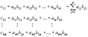
Hence the entry C (i, i) will be 1 whenever A (i, j) = B (j, i) = 1, this is from the definition of matrix multiplication, element by element view, since:
For all entries except when the entry, and at the same time, but since is the transpose of P, then whenever then only when.
Hence this leads to with all other entries in C being zero, i.e.
Question 4
(a)
If A is invertible and AB = AC, then B = C is true.
Because;
This means that; IB = IC, and subsequently B = C
(b)
Suppose:
AC = AB; then:
0 = AB – AC = A (B-C)
If , Note that if we define
Then you can find by multiplying it out that:
Therefore, if we set we find that:
So for this choice of A, just pick any 2×2 matrix for B, and define C = D + B; and automatically, you will find that: AC = A (D + B) = AD + AB = 0 + AB = AB; but C is not = B.
Question 6
Start with the augmented matrix:
Then the only row on the left that doesn’t already look like the identity matrix is the second row; we just need subtract rows 1 and 3 from row 2, which gives:
Hence,
To find, start with the augmented matrix:
Replace the 1st row by half of itself and add half of the 1st row to the 2nd row:
Next, add a third of the second row to the first, add 2/3 the second row to the third, and multiply the second row by 2/3:
Finally, multiply the third row by 3/4, and then add 1/3 of the result to row 1 and add 2/3 of the result to row 2:
Thus,
To find, start with the augmented matrix:
First, switch rows 1 and 3:
Now, subtract row 2 from row 1 and subtract row 3 from row 2:
Thus,
Question 10
For the first choice of A, we write the augmented matrix [A I]:
Then subtracting two times row 1 from row 2 and subtracting three times row 3 from row 2 yields
Hence,
For the second choice of A, write the augmented matrix [A I]:
Subtracting row 1 from rows 2 and 3 yields:
In turn, subtracting row 2 from rows 1 and 3 yields:
Finally, subtracting row 3 from row 2 yields:
Hence,
Question 13
Question 17
The inverse of a lower (upper) triangular matrix is still lower (upper) triangular. Multiplying lower (upper) triangular matrices gives a lower (upper) triangular matrix.
The main diagonal of and are the same as those of and , so we have. By comparing the off-diagonals of, both matrices must be diagonal. , is invertible so.
Then
Question 18
To make the pivot actually occur at f, switch rows 1 and 3:
Now, subtract d/j times row 1 from row 2 and subtract a/f times row 1 from row 3; note:
If e = 0 then the 2nd row is all zeros, which means that there can’t be a pivot in that row. Thus, when A is invertible, it must be the case that e 0. Therefore, a pivot is in the 2nd column, and the entry below can be eliminated through subtraction of times on row 2 from row 3:
If A is to be invertible, it must be the case that c 0. Therefore, the conditions which ensure that A is invertible are:
Turning to B, the matrix becomes:
Then, in order to have a pivot in the 2nd row, it must be the case that
Or, equivalently,
On the other hand, if, so we can switch rows 1 and 2 to get
Then we can eliminate a by subtracting times row 1 from row 2 (note:
Again, if we are to have a pivot in the 2nd row, it must be the case that:
Or, equivalently,
Therefore, either
Question 22
Question 43
The 5 by 5 also has 1s on the diagonal and super-diagonal.
Review Exercises
Question 1.2
Question 1.4
Question 1.10
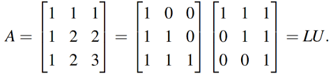
Has L = I and;
A = LU has U = A (pivots on the diagonal);
A = LDU has with 1s on the diagonal.
Question 1.17
Question 1.28
2 by 2; d = 0 not allowed;
d = 1, e = 1; then l = 1, f = 0 is not allowed.
Vector Spaces
Question 2
The answer is: (a), (b) and (e).
Question 3
is the x-axis; is the line through (1, 1); is ; is the line through (-2, 1, 0); is the point (0, 0) in ; the null space is .
Question 14
The subspaces of are itself, lines through (0, 0), and the point (0, 0).
The subspaces of are itself, three-dimensional planes , two-dimensional subspaces , one-dimensional lines through (0, 0, 0), and (0, 0, 0) alone indicate that the smallest subspace containing P and L is either P or .
Question 24
The extra column b enlarges the column space, unless b is already in that space,
1) Introduction
a) Capture the reader’s interest, provide context for the paper, and include a clear thesis statement
2) Purposes of the Articles
a) Article 1 purpose
b) Article 2 purpose
c) Article 3 purpose
d) Commonalities/shared themes between articles
e) Why is that interesting or important?
3) Research Questions
a) Article 1 research questions/hypotheses
b) Article 2 research questions/hypotheses
c) Article 3 research questions/hypotheses
d) Commonalities/shared themes between articles
e) Things to address in this section of the paper: What are the research questions and hypotheses asked by the authors? How do they compare to one another? Why might the differences and similarities be important?
4) Literature Reviews
a) Article 1 themes
b) Article 2 themes
c) Article 3 themes
d) Commonalities/shared themes between articles
e) Conclusions I can draw from the shared themes
f) Things to address in this section of the paper: What are the main themes of each article’s lit review? What do they share in common? What conclusions can you draw from that?
5) Research Participants
a) Article 1 sample
b) Article 2 sample
c) Article 3 sample
d) Commonalities/shared themes between articles
e) Things to address in this section of the paper: Who participated in this study? What is important about the participants? What do the articles have in common?
6) Limitations
a) Article 1 limitations
b) Article 2 limitations
c) Article 3 limitations
d) Commonalities/shared themes between articles
e) Things to address in this section of the paper: What limitations exist in this article? Consider issues with sample, generalizability of results, biases of researchers, etc.
7) Results/Conclusions
a) Article 1 results/conclusions
b) Article 2 results/conclusions
c) Article 3 results/conclusions
d) Commonalities/shared themes between articles
e) Things to address in this section of the paper: What are the results of the studies? What conclusions did the authors draw? What commonalities do you see between articles? Why might that be important? What might that mean?
8) Conclusion
a) What is your conclusion? If you consider all three articles to be a single entity, what conclusions can you draw from their combined research? What is the overall message of the articles? Why is this important? What suggestions might you have for future research, or practical application of this information
SAMPLE ANSWER
1) Introduction
Expanded comparison matrix is undoubtedly the widely used and the most important tool that is used to compare contents of different articles, especially the peer reviewed journal articles on a particular subject. The context of this paper is comparing socialization or networking in higher education. As a result, this paper compares all sections of the three considered articles in order to establish an appropriate comparison matrix.
The three articles considered in this comparison matrix are: Baker & Lattuca (2010); Visser, Visser & Schlosser (2003); and Weidman & Stein (2003) as article 1, 2 and 3 respectively.
2) Purposes of the Articles
a) Article 1: The purpose of this article is to examine how doctorate graduate students are prepared for academic careers, particularly focusing on their academic professional identity development.
b) Article 2: The purpose of this article is to assess current teaching practices and investigate the critical thinking knowledge among faculty, whilst undertaking the identification of exemplary practices in critical thinking teaching.
c) Article 3: The purpose of this article is to study how doctoral students socialize to the academic norms of scholarship and research.
d) The commonalities between the purposes of the considered articles is that they all target students at doctoral level in education, particularly with regards to socialization and networking.
e) The importance of the commonalities is that they allow easy comparison of the obtained results.
3) Research Questions/Hypotheses
a) Article 1: This article hypothesize that there is connection between developmental networks of doctoral students, their graduate experience learning and professional identity development.
b) Article 2: The research question in this article is that, are instructors and students (as lifelong learners and as reflective practitioners) helping our students to become critical thinkers?
c) Article 3: The research question of this article is that, how do doctoral students’ socialize to academic norms of scholarship and research?
d) The commonalities between the purposes of the considered articles is that, they all seek to establish a particular aspect of doctoral students’ socialization.
e) The similarities enable the researcher to compare and contrast the study results.
4) Literature Reviews
a) Article 1: In this article, sociocultural perspectives on higher education learning and network theories are examined with an emphasis on mentoring and social networking theories in addition to evaluating the intersection of sociocultural learning and developmental network theories.
b) Article 2: In this article, the literature is reviewed from the perspective of the factors that affecting integration of critical thinking to higher learning in distance and traditional higher education such as faculty factors, learner factors as well as learner environment factors.
c) Article 3: in this article, various aspects of how socialization theories are discussed in details in order to build up on the proposed theoretical framework.
d) The commonalities between the purposes of the considered articles is that, the three articles adopt the same theoretical or conceptual framework to build on the literature review.
e) The commonalities of the literature reviews is important in providing an overview of how the adopted theoretical or conceptual frameworks are developed.
5) Research Participants
a) Article 1: In this article, the research participants or sample size was 50 doctoral students who were interviewed and most of them have been engaged in various activities of their creativity to either partially or fully evade the need of analyzing, documenting or theorizing their work.
b) Article 2: In this article, the research participants included 66 universities in California (both private and public) from where the research study was carried out.
c) Article 3: In this article, all the 83 doctoral students were included in the study as part of research participants.
d) The commonalities between the purposes of the considered articles is that, the number of participants is almost the same among all the considered articles.
e) Since the number of research participants in all the three articles is relatively the same, it would be easy to compare the results.
6) Limitations
a) Article 1: The limitation in this article is that, the outcomes equation complexity is suggestive of a study that evaluate the influence of conflicting network values, goals and norms with regards to doctoral students without consideration of students at lower education levels or network partners and local contexts.
b) Article 2: In this article, the main limitation is inherent in the research design since the two groups considered in this study are not universally treated because the distance learning group can access all books, whilst the classroom group does not enjoy this privilege.
c) Article 3: In this article, the main limitation is concerned with how the sample size was collected since all the doctoral had to be included with an appropriate method of sampling.
d) The commonalities between the purposes of the considered articles is that, there are delimitations to most of the identified limitations.
e) Identification of the limitations is essential since it enables the appropriate delimitations to be devised.
7) Results/Conclusions
a) Article 1: in this article, the results indicate that oftentimes most of the doctoral students usually achieved a workable equilibrium between their aesthetic and analytic activities, which is envisaged to redefine conceptual and theoretical ideas previously considered as challenges towards inspiration resources.
b) Article 2: The results of this article found that while about 90% of the interviewed instructors claimed that in their instruction critical thinking constitutes the core objective, only 19% of them could succinctly explain the meaning of critical thinking.
c) Article 3: The results of multivariate analysis confirm that, social interaction is important among doctoral students and their departments.
d) The commonalities between the purposes of the considered articles is that, the results of the three articles affirms the need for students in higher education levels to socialize and network.
e) The results obtained in the three articles can be applied in other areas where social interaction or networking among higher education students is considered.
8) Conclusion
It can be concluded that a comparison of the three articles that are considered in this comparison matrix reveals a number of commonalities in almost all sections, particularly with regards to conceptual and theoretical frameworks as well as research designs. A consideration of the three articles combined, it is evident that socialization and networking among students is important for both distant and classroom students. Future research is recommended to determine the envisaged trends in student socialization and networking in future both for classroom and distance students.
The Pearson product-moment correlation coefficient (Pearson’s correlation) is a measure of the strength and direction of association that exists between two variables measured on at least an interval or ratio scale (Ghauri, 2005). From the data set, several variables will be tested to determine if any relationship occurs among the variables under study. The tests will be conducted at a significance level to determine if the possible relationships occur due to chance or a possible relationship.
Assumptions of Pearson’s correlation
1: The two variables should be measured at the interval or ratio level (i.e., they are continuous)
2: There needs to be a linear relationship between the two variables. Whilst there are a number of ways to check whether a linear relationship exists between the two variables, create a scatter plot using SPSS, where one can plot the dependent variable against the independent variable, and then visually inspect the scatter plot to check for linearity. If the relationship displayed in the scatter plot is not linear, either run a non-parametric equivalent to Pearson’s correlation or transform your data, which can be done using SPSS.
3: There should be no significant outliers. Outliers are simply single data points within your data that do not follow the usual pattern (Ghauri, 2005).
Hypothesis Testing
In this study, the relationship between the number of hours worked and the injury rate will be investigated. The following hypothesis was formulated to study the relationship;
H0: The rate of injury is independent from the number of hours worked in the manufacturing locations.
H1: The rate of injury changes (increases or decreases) with the number of hours worked in the manufacturing locations
To test the above hypothesis, Pearson’s correlation test was conducted to establish if there existed any significant relationship between injury rate and the number of hours worked at a 95% confidence interval using SPSS.
Procedure
Load data into SPSS from the excel spreadsheet. From the data editor menu bar, select analyze and from the drop down menu which pops up, choose correlate and then proceed to bivariate correlation. A bivariate correlations window appears where you choose the variable to test from the left hand side box and move them to the right. Highlight on number of hours worked and move it to the right and repeat the same procedure for the injury rate. From the same window, proceed to the correlation coefficients section and select Pearson by checking in the box preceding it. Proceed to the test of significance section and check the two tailed radio button then select ok to conduct the test (Kumar, 2009).
A linear relationship exists between the variables under study is an important assumption in conducting a Pearson’s correlation. To investigate the presence of this relationship, a scatter plot is drawn using SPSS. The procedure involves; from the SPSS data editor menu bar, select graphs then from the drop down menu that appears, choose legacy dialogs then select scatter/dot plot. A dialog box pops up where you select simple scatter and click define. A simple scatter window appears with the variables on the left hand side from where you highlight on hours worked and move it to the x axis box and then choose injury rate and move it to the y axis box. Click ok to produce the scatter plot using SPSS.
The output obtained from the tests conducted is explained below.
Correlations
Hours Worked
InjuryRate
Hours Worked
Pearson Correlation
1
-.636**
Sig. (2-tailed)
.000
N
51
51
InjuryRate
Pearson Correlation
-.636**
1
Sig. (2-tailed)
.000
N
51
51
**. Correlation is significant at the 0.01 level (2-tailed).
Table 1
Decision Rule
Reject H0 if (Creswell, 2003). From table 1 above, p value = 0.000 which is less than 0.05 hence we reject the null hypothesis.
Conclusion
We can conclude that the injury changes (increases or decreases) with the number of hours worked in the manufacturing locations at a 95% level of precision. The Pearson Correlation coefficient posted a result of -0.636 which indicates a strong negative relationship between the injury rate and the number of hours worked. The p value reading of 0.000 confirms that no single outcome occurs due to chance and the test significant. The scatter plot confirms the negative relationship of the 2 variables as indicated by the coefficient (Gay et al, 2009). The scatter plot does not post a perfect relationship of -1 due to the presence of outliers but the strong relationship was confirmed by the scatter dots as shown in figure 1 in the appendix section.
Regression Analysis
Linear regression is the next step up after correlation. It is used when we want to predict the value of a variable based on the value of another variable. The variable we want to predict is called the dependent variable (or sometimes, the outcome variable). The variable we are using to predict the other variable’s value is called the independent variable or sometimes, the predictor variable (Ghauri, 2005).
Assumptions of Regression Analysis
1: The two variables to be studied should be measured at the continuous level (i.e., they are either interval or ratio variables)
2: There needs to be a linear relationship between the two variables. Whilst there are a number of ways to check whether a linear relationship exists between the two variables, one can create a scatter plot using SPSS Statistics where one can plot the dependent variable against the independent variable and then visually inspect the scatter plot to check for linearity.
3: There should be no significant outliers. An outlier is an observed data point that has a dependent variable value that is very different to the value predicted by the regression equation. As such, an outlier will be a point on a scatter plot that is (vertically) far away from the regression line indicating that it has a large residual.
4: There should be independence of observations, which can easily be checked using the Durbin-Watson statistic, which is a simple test to run using SPSS Statistics..
5: Your data needs to show homoscedasticity, which is where the variances along the line of best fit remain similar as you move along the line.
6: Finally, check that the residuals (errors) of the regression line are approximately normally distributed. Two common methods to check this assumption include using either a histogram (with a superimposed normal curve) or a Normal P-P Plot (Ghauri, 2005).
Hypothesis Testing
In this study, the relationship between the number of hours worked and the injury rate will be investigated. The following hypothesis was formulated to study the relationship;
H0: The rate of injury is independent from the number of hours worked in the manufacturing locations.
H1: The rate of injury changes (increases or decreases) with the number of hours worked in the manufacturing locations
To test the above hypothesis, a linear regression or goodness of fit test was conducted to investigate the presence of linear relationship between the 2 variables as stated at 95% level of precision.
Procedure
After loading the data into SPSS, select analyze from the SPSS data editor menu bar. From the drop down menu which appears, choose regression then linear. A dialog box with the variables on the left hand side where injury rate is selected and moved to the dependant variable box while the number of hours worked is moved to the independent variable box. On the right hand side of the same dialog box select plots then move the predictor variable to the x axis and the residuals to the y axis and choose histogram and normal probability plot then click ok to conduct the test (Kumar, 2009). The output obtained is explained below;
Model Summary
Model
R
R Square
Adjusted R Square
Std. Error of the Estimate
1
.636a
.405
.393
1.361737129585175E1
a. Predictors: (Constant), Hours Worked
Table 2
ANOVAb
Model
Sum of Squares
df
Mean Square
F
Sig.
1
Regression
6182.010
1
6182.010
33.338
.000a
Residual
9086.207
49
185.433
Total
15268.217
50
a. Predictors: (Constant), Hours Worked
b. Dependent Variable: Injury Rate
Table 3
Coefficientsa
Model
Un-standardized Coefficients
Standardized Coefficients
t
Sig.
B
Std. Error
Beta
1
(Constant)
50.809
6.459
7.866
.000
Hours Worked
.000
.000
-.636
-5.774
.000
a. Dependent Variable: Injury Rate
Table 4
Decision Rule
Reject H0 if (Creswell, 2003). From table 1 above, p value = 0.000 which is less than 0.05 hence we reject the null hypothesis.
Conclusion
We can conclude that the injury changes (increases or decreases) with the number of hours worked in the manufacturing locations at a 95% level of precision. The linear regression model posted an R value of 0.636 which indicates a strong relationship between the injury rate and the number of hours worked as shown in table 2. The R squared reading of .405 indicated that 40% of the variation in the injury rate can be explained by the number of hours worked. Table 3 gives F statistic (F 50= 33.338) which is a measure of the absolute fit of the model to the data. Here, the F-test outcome is highly significant (less than .001, as you can see in the last column), so the model does fit the data. A straight line, depicting a linear relationship, described the relationship between these two variables. Table 4 gives the coefficients of the model as follows; Injury Rate = 50.809+ 0 hours worked (Kumar, 2009). The histogram with a superimposed normal curve and the normal p- p plot confirm the assumption that the residuals (errors) of the regression line are approximately normally distributed shown in figure 2 & 3 in the appendix section
Discriminant analysis which highly related to regression analysis was not the best test to conduct since it is very robust to violations of assumptions and in turn, it can yield less powerful statistics when assumptions are violated (Gay et al, 2009).
References
Creswell, J. W. (2003). Qualitative, quantitative, and mixed methods approaches(2nd ed.). Thousand Oaks, CA: Sage.
Gay, L,R., Mills, E. G., & Airasian, P.,(2009). Educational Research: Competencies for Analysis and Applications (10th ed.)
Ghauri, P. (2005). Research Methods in Business Studies: a Practical Guide.
Kumar, R. (2009). Research Methodology: A step-by-step Guide for Beginners. Greater Kalash: Sage Publications.
Appendix
Figure 1
Figure 2
Figure 3
We can write this or a similar paper for you! Simply fill the order form!