Statistics Analysis Research Paper Available

Statistics Analysis Research Paper

Order Instructions:

Please let me know how many pages will be.
I will email the task and other related documents later.
Thank you very much.

SAMPLE ANSWER

Question 1

Conduct a one-way ANOVA to investigate the relationship between hair color and social extroversion. Be sure to conduct appropriate post hoc tests. On the output, identify the following:

F ratio for the group effect
Sums of squares for the hair color effect
Mean for redheads
P value for the hair color effect

Table 1: Definition of variables

Variable

Definition

Hair Color

1 = Blond

2 = Brunet

3 = Red Head

Social Extroversion

A measure of social extroversion

According to Kumar (2008), the following steps were followed to carry out the test. On the data editor menu bar, Click analyze then a drop down menu pops and general linear model is chosen then univariate. In the Univariate dialog box, choose extroversion then move it to the dependant variable box and Click on hair color and move it to the fixed factor(s) box. Click options and from the dialog box which appears, click hair color on the factor(s) and factor interactions box and move it to the display means for box. In the display box, click homogeneity tests, estimates of effect size, and descriptive statistics. In the factor(s) box, choose hair color and move it to the post hoc tests for box. Click turkey and R-E-G-W-G in the equal variances assumed box. Also click dunnet’s c in the equal variances not assumed box.

Descriptive Statistics
Dependent Variable: Social Extroversion
Hair Color	Mean	Std. Deviation	N
Blond	5.17	2.787	6
Brunet	3.67	1.211	6
Redhead	2.33	1.033	6
Total	3.72	2.109	18

Table 2

Levene’s Test of Equality of Error Variances^a
Dependent Variable:Social Extroversion
F	df1	df2	Sig.
1.520	2	15	.250
Tests the null hypothesis that the error variance of the dependent variable is equal across groups. Table 3

Tests of Between-Subjects Effects
Dependent Variable:Social Extroversion
Source	Type III Sum of Squares	df	Mean Square	F	Sig.	Partial Eta Squared
Corrected Model	24.111^a	2	12.056	3.511	.056	.319
Intercept	249.389	1	249.389	72.638	.000	.829
hair	24.111	2	12.056	3.511	.056	.319
Error	51.500	15	3.433
Total	325.000	18
Corrected Total	75.611	17
a. R Squared = .319 (Adjusted R Squared = .228)

Table 4

A one-way analysis of variance was performed to evaluate the relationship between hair color and social extroversion. Hair food was the independent factor and it included three levels i.e. blond, brunet and red head. Measure of social extroversion was the dependant variable .The ANOVA test conducted was significant at the 0.05 level, F (2, 15) = 3.511, p = 0.056, ms _error= 3.433 (Ghauri, et al. 2005).

From the above output;

a). F ratio, F (2, 15) = 3.511

b). p value, p = 0.056

c). Sum of squares for hair color, SS = 24.111

d). Mean for red heads, m = 2.33

Question 2

Effect size for the relationship between hair color and extroversion

According to Gay, et al, (2009) the strength of the relationship between hair color and the measure of social extroversion as assessed by n², was strong with hair color accounting for 32% of the variance of the dependent variable.

Pair wise differences were evaluated through conducting follow-up tests. Variances among the 3 groups range from 1.067 to 7.8 hence we assume that equal variances were not assumed and we therefore evaluate results for the Dunnett’s C test as a post hoc comparison test. From table 4 below, there was a significant difference in the means between the brunet and the blond group and also between redhead and blond group but no significant difference between brunet and red head at a 95%confidence interval.

95% confidence intervals of pair wise differences in mean measure of social extroversion

Hair Color

Blond Brunet

Blond

Brunet

Red Head

5.17

3.67

2.33

2.787

1.211

1.033

(-2.54, 5.54)

(-1.11, 6.78) (-0.78, 3.45)

Table 5

Question 3

A box plot to display the differences among the distribution for the 3 hair color groups.

To create the box plot, click graphs from the data editor menu bar. Then choose legacy dialogs and click on box plots from the drop down menu which appears. Choose simple then define the variables and click ok (Kumar, 2008).

Figure 1 (Source: SPSS output)

References

Ghauri, P., Granhaug, K. and Kristianslund, I.,(2005). Research Methods in Business Studies: a Practical Guide.

Kumar, R. (2008). Research Methodology: A step-by-step Guide for Beginners. Greater Kalash: Sage Publications

Gay, L,R., Mills, E. G., Airasian, P.,(2009). Educational Research: Competencies for Analysis and Applications (10^th ed.)

Appendix

Multiple Comparisons
Dependent Variable: Social Extroversion
	(I) Hair Color	(J) Hair Color	Mean Difference (I-J)	Std. Error	95% Confidence Interval
	(I) Hair Color	(J) Hair Color	Mean Difference (I-J)	Std. Error	Lower Bound	Upper Bound
Dunnett C	Blond	Brunet	1.50	1.241	-2.54	5.54
	Blond	Redhead	2.83	1.213	-1.11	6.78
	Brunet	Blond	-1.50	1.241	-5.54	2.54
	Brunet	Redhead	1.33	.650	-.78	3.45
	Redhead	Blond	-2.83	1.213	-6.78	1.11
	Redhead	Brunet	-1.33	.650	-3.45	.78
Based on observed means. The error term is Mean Square(Error) = 3.433.

Table 6

Social Extroversion
	Hair Color	N	Subset
	Hair Color	N	1	2
Tukey B^a	Redhead	6	2.33
	Brunet	6	3.67	3.67
	Blond	6		5.17
Ryan-Einot-Gabriel-Welsch Range^b	Redhead	6	2.33
	Brunet	6	3.67	3.67
	Blond	6		5.17
	Sig.		.232	.181
Means for groups in homogeneous subsets are displayed. Based on observed means. The error term is Mean Square(Error) = 3.433.
a. Uses Harmonic Mean Sample Size = 6.000.
b. Alpha = .05.

Table 7

We can write this or a similar paper for you! Simply fill the order form!

Statistical Essay Paper Available Here

Statistical essay

The purpose of the Final Exam is to assess your understanding of the main statistical concepts covered in this course. Below are three essay questions. All of your responses should be included in a single Word document for submission.
Please include the following general headings for each section of the written exam within your Word document:
Part I: Essay Questions
1. Essay 1
2. Essay 2
3. Essay 3
Your complete Word document must include a title page with the following:
1. Student’s name
2. Course name and number
3. Instructor’s name
4. Date submitted
Part I: Essay Questions
There are three essay questions in this section. You must answer all three questions. The length of each essay should be one to two double-spaced pages
(excluding title and reference pages). Use 12-point font and format your paper with regular 1-inch margins. Do not include the essay prompt in your document.
It will not count toward the length requirement for your essays.

Essay 1
A group of researchers conducted an experiment to determine which vaccine is more effective for preventing getting the flu. They tested two different types of vaccines: a shot and a nasal spray. To test the effectiveness, 1000 participants were randomly selected with 500 people getting the shot and 500 the nasal spray. Of the 500 people were treated with the shot, 80 developed the flu and 420 did not. Of the people who were treated with the nasal spray, 120 people developed the flu and 380 did not. The level of significance was set at .05. The proportion of people who were treated with the shot who developed the flu =.16, and the proportion of the people who were treated with the nasal spray was .24. The calculated p value = .0008. For this essay, describe the statistical approaches (e.g., identify the hypotheses and research methods) used in this excerpt from a research study.
Interpret the statistical results and examine the limitations of the statistical methods. Finally, evaluate the research study as a whole and apply what you have learned about hypothesis testing and inferential statistics by discussing how you might conduct a follow-up study.

Your essay must address the following points:

Describe the research question for this experiment.#9702;What were the null and alternative hypotheses?#9702;Were the results of this test statistically significant?
#9702;If so, why were they significant?
Would the researchers reject or fail to reject the null hypothesis?
Do the results provide sufficient evidence to support the alternative hypothesis?
Was the sample appropriate for this study? Explain your answer.
What are some possible limitations to this study?
Discuss how you would conduct a follow up study to this one. Explain your answer.
Describe the difference between practical and statistical significance.

Essay 2
A researcher has investigated the relationship between IQ and grade point average (GPA) and found the correlation to be .75.
For this essay, critique the results and interpretation of a correlational study.

Evaluate the correlational result and identify the strength of the correlation.
Examine the assumptions and limitations of the possible connection between the researcher?s chosen variables.
Identify and describe other statistical tests that could be used to study this relationship.

Your essay response must address the following questions:

How strong is this correlation? ;#9702;Is this a positive or negative correlation?
#9702;What does this correlation mean?
Does this correlation imply that individuals with high Intelligence Quotients (IQ) have high Grade Point Averages (GPA)?
Does this correlation provide evidence that high IQ causes GPA to go higher? #9702;What other variables might be influencing this relationship?
What is the connection between correlation and causation?
What are some of the factors that affect the size of this correlation?
Is correlation a good test for predicting GPA? #9702; If not, what statistical tests should a researcher use, and why?

Essay 3
A researcher has recorded the reaction times of 20 individuals on a memory assessment. The following table indicates the individual times:
2.2
4.7
7.3
4.1
9.5
15.2
4.3
9.5
2.7
3.1
9.2
2.9
8.2
7.6
3.5
2.5
9.3
4.8
8.5
8.1
In this essay, demonstrate your ability to organize data into meaningful sets, calculate basic descriptive statistics, interpret the results, and evaluate
the effects of outliers and changes in the variables. You may use Excel, one of the many free online descriptive statistics calculators, or calculate the
values by hand and/or with a calculator.
Next, separate the data into two groups of 10; one group will be the lower reaction times, and the second group will be the higher reaction times. Then,
address the following points in your essay response:
Calculate the sum, mean, mode, median, standard deviation, range, skew, and kurtosis for each group.
How do the two groups differ?
Are there any outliers in either data group?
What effect does an outlier have on a sample?
Lastly, double each sample by repeating the same 10 data points in each group. You will have a total of 20 data points for each group. After completing this,
address the following in your essay response:
Calculate the following for the new data groups: sum, mean, mode, median, standard deviation, range, skew, and kurtosis.
Did any of the values change?
How does sample size affect those values?

We can write this or a similar paper for you! Simply fill the order form!

Multivariate Data Analysis( Short computational exercise)

Multivariate Data Analysis

Load the data into the SPSS statistics software package, and answer the following questions.
1. Is there any evidence of an association between occupational status and the number of visits to the Gymnasium during the past four weeks? Carry out an
appropriate hypothesis test.
2. Is there any evidence that the average customer satisfaction score is age-dependent? Carry out an appropriate hypothesis test.
3. The Gymnasium management have calculated that a monthly membership fee of at least £75 will be required to cover the investment and running costs of the upgraded Gymnasium. Test the null hypothesis that the mean willingness-to-pay for membership of the upgraded Gymnasium is at least £75, against the one-sided alternative hypothesis that the mean willingness to pay is less than £75.
4. Test whether there is any evidence of a difference between the willingness-to-pay for membership of the upgraded Gymnasium of male and female customers.
5. Estimate a two-variable linear regression to describe the relationship between household weekly net income and willingness-to-pay for membership of the upgraded Gymnasium. According to this regression, what is the estimated willingness-to-pay of a customer with a household weekly net income of £300?
6. Estimate a multiple regression in which willingness-to-pay for membership of the upgraded Gymnasium is explained by the following characteristics: gender (male/female), occupational status, and household weekly net income.
(i) Comment on the significance of each of these characteristics as determinants of willingness-to-pay.
(ii) Comment briefly on the comparison between the multiple regression estimated in Q6 and the two-variable linear regression estimated in Q5.
(iii) What is the estimated willingness-to-pay of a male self-employed customer with a household weekly net income of £500?
(iv) What is the estimated willingness-to-pay of a female employed customer with a household weekly net income of £400?

We can write this or a similar paper for you! Simply fill the order form!

Cross Tabulation Application Assignment

Cross Tabulation

Cross Tabulation Application Assignment

Order Instructions:

Application: Cross Tabulation

Variable relationships are very important in quantitative research. They tell researchers what effect different variables have upon one another. One of the easiest ways to display relationships between variables is through a cross-tabulation (cross-tab). A cross-tab is simply a chart that shows frequency or distribution of one or more variables for every category of another variable. Stated another way, a cross-tab is a joint frequency distribution of observations on two or more sets of variables. These statistical observations can be presented by numeric frequency, percentages, or both, depending on which is most useful given the specific data context.??For this Application Assignment, perform a cross-tabulation on the data provided in the handout “Week 10 Dataset” such that property crime is displayed as a rate per student population. Though Excel is not the only software that can be used to perform a cross-tabulation, it is used here because it is a widely available program. The handout entitled, “Cross-Tabulation in Excel” contains instructions on how to complete the task in Excel using two different methods.??The assignment (2–3 pages):

• Using Excel, perform a cross tabulation on the data provided in the Week 10 dataset.

• Explain what you can conclude from the output of the cross tabulation.

• Include your outputs in your Application Assignment document. (Copy and paste them from Excel into your Word doc.)

Support your Application Assignment with specific references to all resources used in its preparation. You are to provide a reference list for all resources, including those in the Learning Resources for this course.

Note: Please use the course text as one of the references for this assignment, AND the other articles on the attached files sent by email.

SAMPLE ANSWER

The Pivot table below, shows the total crimes and various categories of crimes committed in each college and totals for all the colleges. The information could help college authorities to know which crimes recur frequently.

College	Sum of Crime Total	Sum of Forcible Rape	Sum of Aggravated Assault	Sum of Arson	Sum of Property Crime
Abalone University	35	5	12	1	17
Franklinville College	4	0	2	0	2
Marie Louis College	14	2	4	0	8
Robert Long College	9	0	1	0	8
Simon State	42	3	5	1	33
Grand Total	104	10	24	2	68

Table I

(Jelen, 2010)

The pivot table below shows student enrolment and the number of crimes committed in each college

Table II

College	Sum of Student enrolment	Sum of Crime Total
Abalone University	10486	35
Franklinville College	989	4
Marie Louis College	2301	14
Robert Long College	3467	9
Simon State	20573	42
Grand Total	37816	104

(Jelen, 2010)

Table III

College	Sum of Student Enrollment	Sum of Crime Total	Crime total as a percentage of student enrollment
Abalone University	10486	35	0.33%
Franklinville College	989	4	0.40%
Marie Louis College	2301	14	0.61%
Robert Long College	3467	9	0.26%
Simon State	20573	42	0.20%
Grand Total	37816	104

The pivot table below shows the grand totals of all the categories of crimes, crime totals and student enrolment arranged in a descending order

Table IV

College	Sum of Student Enrolment	Sum of Crime Total	Sum of Forcible Rape	Sum of Aggravated Assault	Sum of Arson	Sum of Property Crime
Simon State	20573	42	3	5	1	33
Abalone University	10486	35	5	12	1	17
Robert Long College	3467	9	0	1	0	8
Marie Louis College	2301	14	2	4	0	8
Franklinville College	989	4	0	2	0	2
Grand Total	37816	104	10	24	2	68

(Jelen, 2014)

The pivot table below indicates the various categories of crime totals, student enrolment, and various categories of crimes as a percentage of the grand total in each category.

Table V

College	Sum of Student Enrollment	Sum of Crime Total	Sum of Forcible Rape	Sum of Aggravated Assault	Sum of Arson	Sum of Property Crime
Abalone University	27.73%	33.65%	50.00%	50.00%	50.00%	25.00%
Franklinville College	2.62%	3.85%	0.00%	8.33%	0.00%	2.94%
Marie Louis College	6.08%	13.46%	20.00%	16.67%	0.00%	11.76%
Robert Long College	9.17%	8.65%	0.00%	4.17%	0.00%	11.76%
Simon State	54.40%	40.38%	30.00%	20.83%	50.00%	48.53%
Grand Total	100.00%	100.00%	100.00%	100.00%	100.00%	100.00%

(Jelen, 2010)

Report of findings

Table I above shows the total crimes committed in all the colleges which was 104 in total.It also shows the total number of crimes committed in each category of crimes. Table I shows that property crimes were higher than all other crimes at 64 followed by aggravated assault at 24, then forcible rape at 10. The least number of crimes committed at the colleges was arson at only 2 incidences. College administrators can therefore put in place measures to address property crimes which are likely to recur more frequently than the other categories of crimes. Table II shows the relationship between student enrollment and the number of crimes committed. From Table II, it can be observed that the higher the student enrolment the higher the numbers of crimes are committed. For example Simon State with a student enrolment of 20,573 recorded the highest number of crimes at 42 whereas Franklinville College with an enrolment of 989 had only 4 crime incidences. However, this information could be misleading judging by the percentage number of crimes per student enrolment as shown in Table III. Marie Louis College which had a student enrolment of 2301 has a higher percentage of crime occurrences at 0.61% as compared to Simon State which had 0.20% but with a higher student enrollment of 20,573. Franklinville College has a crime incidence ratio of 0.40% to student enrollment. If the same ratio at Franklinville College and Marie Louis College was applied to Simon State, then Simon State would have recorded higher crime incidences than the 42 incidences recorded. The problem of crime is more severe in Marie Louis College than in the colleges with higher enrollment.

Table IV shows the college arranged in an ascending order depending on the crime rates and student enrolment. At the top of the table is Simon State which had the highest number of student enrolment and the highest incidences of crimes followed by Abalone University and so on. The last college is Franklinville College which had the least student enrolment and the least number of crimes recorded. Table V presents the percentage number of crimes, student enrolment and various categories as a total for each category. From the table Simon State had the highest number of student enrolment at 54.40% whereas Franklinville College had the least at 2.62%. Simon State also recorded the highest incidences of crime at 40.38% whereas Franklinville College recorded the least number of crimes of the total crimes recorded in all the colleges at 3.85%.Abalone university recorded the highest number of forcible rape, aggravated assault and arson crimes as compared to other colleges at 50.00% of all crimes committed in these crime categories. Simon State recorded the highest number of property crimes of all other colleges at 48.53%. Abalone University administrators should check forcible rape, aggravated assault and arson because they are more likely to recur. Simon State should focus more on tackling property crime to bring down crime incidences within its precincts.

References

Jelen, B. (2014). Excel 2013 pivot tables offer distinct count. Strategic Finance, 96(4), 52-53 Retrieved from http://search.proquest.com/docview/1614145336?accountid=45049

Jelen, B. (2010). Filtering multiple pivot tables in excel 2010. Strategic Finance, 92(3), 52-53 Retrieved from http://search.proquest.com/docview/751221731?accountid=45049

We can write this or a similar paper for you! Simply fill the order form!

Measures of Central Tendency Application

Measures of Central Tendency

Measures of Central Tendency Application

Order Instructions:

see the attached files:

Application: Measures of Central Tendency

Measures of central tendency may be familiar to you from prior math classes you have taken. Consider the summary of these terms below:

The mean is the average of all numbers in a set of data.
The mode is the number in a dataset that most frequently occurs.
The median is the number that falls in the middle of the numbers in a given set when those numbers are placed in rank order.
The standard deviation tells how far the numbers in a given data set deviate from the mean of that set. In other words, it tells whether the numbers in the dataset are generally close together or far apart.

These measures are simple but extremely valuable for all social scientists, including criminal justice researchers. They are summary statistics, which provide useful information about the study sample and allow researchers to compare multiple data sets.  For this Application Assignment, use the following statistics:  The total population of the Battawba metropolitan area was 5,604,383 persons in 2011. For that year, the following burglary rates were reported in the localities within this metropolitan area:

Area	Number of Burglaries Reported
City of Battawba	2,563
City of Wineburg	734
City of Lakeville	301
City of Drake	1,482
City of Valmer	231
City of Chase Abbey	857
City of Southmetro	644
City of Collington	1026
City of Williamson	644
City of New Batten	159

The assignment (2–3 pages):

Calculate the mean, median, mode, and standard deviation for the burglary statistics provided on the metropolitan area of Battawba.
Explain your interpretation of the measures of central tendency and standard deviation for burglary rates in the Battawba metropolitan area (i.e., what they can tell you about who is committing crime and where it is being committed).

SAMPLE ANSWER

The mean of a distribution of values is obtained by adding all of the values and dividing the sum by the number (Nor n) of values. The mean score is the typical performance level of all the units sampled. The mean for the burglaries reported in Battawba metropolitan area is given as

= 864.1= 864 cases

This means that on average, 864 incidences of burglaries are reported with a standard deviation of 717 in the Battawba Metropolitan area with the city of Battawba, Wineburg, Drake,Chase Abbey, Southmetro, Collington Williamson experiencing the highest incidences.

The median represents the middle point of a distribution of data. It is the point at which exactly half of the observed values in the distribution are higher and half of the observed values are lower. The Median value for burglaries in Battawba metropolitan area is

MD=689 cases

This implies that 50% of Battawba metropolitan area has a lower than 689 cases of burglary report and 50% of Battawba metropolitan area has a higher than 689 cases of burglary report cases (Peavy, Dyal, Eddins, & Centers for Disease Control (U.S.), 1981).

The mode (Mo) is the simplest measure of central tendency and is easy to derive. The

Mode is observed rather than computed. The mode (Mo) of a distribution of values is the value

which occurs most often . The distribution of a given data can either be unimodal if it has only one mode or bimodal if it has two modes. Other distribution has more than two modes. For the case of burglaries in Battawba metropolitan area is, the mode is

Mode = 644 cases

This data has only one mode and its distribution can be said to be unimodal

This value implies that the number of burglary incidences that are frequently reported in Battawba metropolitan area is 644 cases and most of these are reported in the city of Southmetro and the city of Williamson. This cities are now our modal cities. These are the cities where most cases of burglary are frequently reported.

The standard deviation is given as Square root of variance (Grigg, & Transport and Road Research Laboratory, 1981)

Var (x) = 513689

Sd (x) = 716.721= 717

According to PL,Chebyshev (1821-1894), for any number k greater than 1, atleast (1-1/k²) of the measurements fall within standard deviation of the mean. That is within the interval (µ-ks, µ+ks)

Where µ is the mean of the sample or population and s is the variance of the sample data or population. For the case of burglaries in Battawba metropolitan area for k=1, that is one standard deviation, the interval is (147,1581). This indicates that about 100% of the burglary cases reported fall within one standard deviation, hence, there is less variations in the burglaries in the cities, except for the Battawba city which falls outside the interval. In conclusion, variation within the data is small. Most of the cases reported are concentrated around the mean

References

Peavy, J. V., Dyal, W. W., Eddins, D. L., & Centers for Disease Control (U.S.). (1981).Descriptive statistics: Measures of central tendency and dispersion. Atlanta, Ga: U.S. Dept. of Health and Human Services/Public Health Service, Centers for Disease Control.

Grigg, A. O., & Transport and Road Research Laboratory. (1981). Rating scales: Measures of central tendency and sample sizes. Crowthorne, Berkshire: Transport and Road Research Laboratory.

Bridges, J. (1961). Statistics for Selected Secondary-School Students. Education Digest, 27(3), 52-53.

We can write this or a similar paper for you! Simply fill the order form!

R studio Data Analyzing Assignment

R studio Data Analyzing

Data analysis project “dry run”
Format: Please submit a SINGLE document (docx or pdf) containing your answers to all questions, with your complete R script copied and pasted to the end of the document. Your R script should include your name, the date, a brief description or title, and all the commands needed to create ALL the output for your
assignment, as well as comments (#). Please make sure not to repeat any errors noted in your previous assignments.

Introduction: This assignment is a “dry run” of the regressions you plan to use in the final report of your Data Analysis Project. Your regressions should be
presented in one or two mtables in a document, with accompanying discussion of the specifications and results. The document should discuss every regression in your table(s).
Read the final project assignment so you know what you need to do. The overall task for the final project is:
Write and submit a report, backed up by statistical analysis of the 2011 ACS data set, exploring the gender earnings gap among college graduates. Is there currently a gap between the earnings of male and female workers? Does that gap persist when we control for other worker characteristics correlated with earnings? Does the size of the gender gap vary by worker characteristics?
For this assignment (#8), do the following:
In a paragraph or two, describe your regression model of earnings: How do you plan to use regression(s) to estimate the gender gap and its determinants? What are your key variables (dependent variable and regressors)? How do you plan to determine whether the gender gap varies by worker characteristics?
You should start with a base specification. You may, if you like, start with a version of one of Weinberger’s regressions, augmented as you see fit.
Run a few alternative specifications to examine the impact of additional regressors/ controls, nonlinear specifications, interactions, etc. You could also
consider running separate regressions for males and females. Explain the choices you have made. Discuss the results: Make sure to assess the statistical
significance and magnitude of the effects. What do you learn about the gender gap and its determinants? Make sure your text refers to and interprets each
regression. Number or label your regression columns and refer to specific regressions by number when discussing them in the text.
Be prepared to discuss what you did in the lab class.
You will be free to change your regressions for your final report… this is just to get you started.
below is the final project which related in top assignment
1. A written essay, maximum of 2000 words, double-spaced, with the following components:
Executive summary: One paragraph summarizing your research questions and findings
Short introduction and overview of the issue of the gender earnings gap, drawing on your readings, and an overview of the ACS data set
Description of your regression model of earnings: How do you plan to use regression(s) to estimate the gender gap and its determinants? What are your key
variables (dependent variable and regressors)? How do you plan to determine whether the gender gap varies by worker characteristics?
Discussion of regression results (refer to regression tables)
Base specification(s): You could, for example, start with something like Weinberger’s model (1), but you are free to do what you like.
Alternative specifications and extensions: Try additional variables or different functional forms; consider whether the gender gap varies by worker
characteristics. Explain briefly why you did what you did.
Discuss your findings:
What is your preferred specification?
What do your regressions tell you about the gender gap? Do your results shed any light on the role of qualifications vs. discrimination?
Discuss whether your findings are consistent under alternative specifications.
Internal and external validity: Discuss potential threats to the internal and external validity of your analysis, especially potential sources of bias. Use
Chapters 8 and 9 of Stock and Watson as your guide.
Conclusions
2. Tables and figures:
At the end of the written essay, add your tables and figures. You may include up to two (2) tables of regression results, each table containing no more than six (6) regressions, and up to four (4) figures (plots). These are maxima: You DO NOT have to include this many! Please format the tables so the columns line up and I can easily read them (it helps to use a font like Courier or Lucida for the tables).
This assignment is using acs_data_bach.csv data. and i will upload the tutorial documents provided by the professor, you can refer to that.

We can write this or a similar paper for you! Simply fill the order form!

Interpreting Data Outputs Research Paper

Interpreting Data Outputs

Order Instructions:

Application: Interpreting Data Outputs
Qualitative data analysis (QDA) is the range of processes and procedures whereby raw data are converted into some form of explanation, understanding, or interpretation of the people and situations being investigated. QDA is usually based on an interpretative philosophy to give meaning to collected data. As with all data, analysis and interpretation are required to bring order and understanding to it. After all, a set of numbers or lists of observations are useless without an explanation of why they are important. This requires creativity, discipline, and a systematic approach—there is no single or best way. The best process for a given research situation will depend on the questions that need to be answered and the needs of those who will use the information.

For this Application Assignment, you interpret the outputs of qualitative analyses by examining which variables are significant and what you can conclude from the outputs. Use the qualitative results in the article, “Why Rape Survivors Participate in the Criminal Justice System” for this assignment.
The assignment (2–3 pages):
• Explain your interpretation of the qualitative results in the article, “Why Rape Survivors Participate in the Criminal Justice System,” including which variables are most significant and the conclusions you can draw about the significant variables you identified.

SAMPLE ANSWER

Interpreting Data Outputs

The results for this research are divided into two categories: those factors that influence reporting and those that are influential in the continuing of the investigational process. Respondents under these two categories had different reasons as portrayed in their responses. To be able to identify the most significant variables in this data collected and then be able to draw valid conclusions, it is important to first to look into and explain the qualitative results as displayed in the research findings.

Factors Influencing Reporting

There are three primary factors identified by the respondents as the reasons why the rape victims report the rape cases. These included to prevent additional rapes by the offender and to send a warning to the other people who were thinking of committing a similar crime. Others reported because they were encouraged by others to report the case to the police. The last group of people were those who said that they were never actually given a chance to report as the reports were given to the police by other people without their consent (Bachman & Schutt, 2013). The victims whose main reason for reporting was to bar the offenders from doing the same atrocity to themselves or to other women formed the majority, which was almost half of the total responses received. Those who were encouraged by their colleagues to report formed the second largest group as they were slightly past the quarter mark of the total responses, and the rest are those whose reports reached the police without their knowledge.

Influential Factors in Continuing With the Investigational Process

This part also attracted divergent views from the participants. The researcher wanted to know what made the respondents to participate in the process of investigation into the rape cases even as others shied away from the process. Just like in the first category, majority of the respondents here said they did it purposely to protect others from the suffering they went through after the rape. The second group of participants in this category noted that their reason for continued participation in the investigational process was that they had gained confidence on the strength of their case especially after they had interacted with such stakeholders like the police and the forensic nurse examiner. The continued participation of another group was inspired by the treatment they received from the system personnel. The last group in this category noted that they continuously participated because they had no other choice. All these reasons by the different groups should be taken into consideration and not be actually considered as mutually exclusive (Starzynski, Ullman, Filipas & Townsend, 2005).

Conclusion

Rape victims could either report the rape cases or not. Those who report are always inspired to do so by certain factors. Some were also coaxed by others to do so. There are even others who are reluctant up to that point when others take it upon their responsibility to report their predicament. There are also those victims who could choose to continue participating in the investigational process after the report and others who chose to terminate the case by refusing to participate. As has been seen above, those who chose to pursue the case to the end had different reasons to do. The results would thus be useful in drawing conclusions and recommendations on the topic under research.

References

Bachman, R. & Schutt, R. K. (2013). The Practice of Research in Criminology and Criminal Justice (5^th ed.). New York: Sage Publications.

Starzynski, L.L., Ullman, S.E., Filipas, H.H. & Townsend, S.M. (2005). Correlates of women’s sexual assault disclosure to informal and formal support sources. Violence and Victims, 20, 417–432.

We can write this or a similar paper for you! Simply fill the order form!

Role of p-values and confidence intervals

Role of p-values and confidence intervals within epidemiological research

Order Instructions:

Week 6

Epidemiologists control for variables such as confounding and random error by carefully developing research studies. Although there are not guarantees to eliminate or reduce all possible errors, it is important to minimize their effects.

For this Discussion, review your readings from this week. Then addressing the following:
•
• Identify the role of p-values and confidence intervals within epidemiological research and provide examples of how these are used to interpret research findings.
•
• Discuss the effect sample size has on p-values and confidence intervals and how this affects interpretation of statistical results.

SAMPLE ANSWER

Role of p-values and confidence intervals

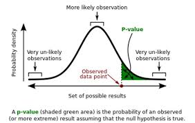
Confidence intervals and p-values are reported in almost every epidemiological research and are used in interpreting statistical analysis results. These measures are used by medical investigators and researchers to answer such questions as: “are the results significant?” or “is the hypothesis accepted?” Epidemiological researchers do not have to worry about testing the significance of results when carrying out statistical researches because they can depend on the p-value and the confidence interval. The p-value is the probability of a value that is similarly extreme or even more extreme as the one in the study if the hypothesis is true. Confidence interval on the other hand can be defined as is an array of values within which there is reasonable confidence that the parameter of the population lies. The reporting of confidence intervals and p-values basically follows that testing of hypothesis or significance, (Bland & Peacock, 2012).

For instance, when testing a hypothesis using the p-value, the particular cutoff or level of significance (conventionally 0.05) is used to test whether values are significant or not; those less are significant, while those above are not. For instance in the study of differences in low birth weight prevalence between singletons and multiple pregnancies, the p value can be used to “endorse” the hypothesis that there is a difference. For the confidence interval, consider a test for difference in mean sugar reduction between a standard hypoglycemic and a new drug. The null hypothesis in this case should state that there is no difference in the blood sugar reduction mean; that can be accepted or rejected, (Gardner& Altman, 2013).

P-values and confidence intervals tend to decrease in size with an increase in sample size unless the null hypothesis is true. As the sample size increases, for the case of the p-value, there is an increased certainty on where the proportion mean might be, and hence large samples are more consistent with smaller ranges of possible population values. For the confidence interval, a larger sample size means a decreased error margin. The effect this has on interpretation of results is that larger samples report small marginal errors and the certainty of finding the true population parameter increases, hence the certainty of the results increases too, (Houle, 2007).

References

Bland M, Peacock J. (2012). Interpreting statistics with confidence. The Obstetrician and Gynaecologist;4:176–180

Gardner MJ, Altman DG. (2013). Confidence intervals rather than P-values: estimation rather than hypothesis testing. Br Med J. 292:746–750

Houle TT. (2007). Importance of effect sizes for the accumulation of knowledge. Anesthesiology. 106:415–417

We can write this or a similar paper for you! Simply fill the order form!

GDP Per Capita and Life Expectancy

GDP Per Capita and Life Expectancy Order Instructions:

Question 2 A

GDP Per Capita and Life Expectancy Sample Answer

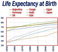
Run the following simple linear regression function on GDP per Capita and life expectancy. Present your regression table along with the interpretation of the intercept and slope coefficients. Additionally, conduct a hypothesis test to see if having 5 extra years of life expectancy could increase GDP per capita by more than $20,000. Show all steps for the hypothesis test and use

Adjusted R squared is a coefficient of determination, which tells us the variation in the dependent variable due to changes in the independent variable. From the findings in the above table, the value of adjusted R squared was 0.25, an indication that there was a variation of 25.1% GDP per Capita due to life expectancy at 95% confidence interval. This shows that 25.1 % changes in GDP can be caused by changes in life expectancy. R is the correlation coefficient, which shows the relationship between the study variables. From the findings shown in the table above, there was a weak relationship between the variables, therefore, at 95%, the hypothesis is rejected as shown by sig. of 0.111, which is beyond 0.005.

R	203
R Square	0.41
Adjusted R	0.25
Stardard Error	2251.71765
Observation	62

ANOVA	df	ss	ms	f	Sig

Regression	1	1.12111E	1.33E+07	2.617	0.111
Residual	61	3.09111E	5070232.4
Total	62	3.2121E


	coefficient	Stardard Error	P value	Lower 95%	Upper 95%
Intercept	-5968.296	4294.492	0.17	0.021	0.081
LIFEEXP	91.344	56.47	0.111	0.412	567

The constant is -5968.296 and the slope of 91.334, therefore, conduct a hypothesis test to see if having 5 extra years expectancy could increase GDP per capita by more than $20,000 and using the equation of the line,,, Y = -5968.296 + 91.334(5 years),,which is – 5511.626 and therefore by 5 extra years the GDP will have decreased by – 5511.626 and this in line with the rejection of the hypothesis.

Based on the multiple regression results you had in Part 3a, test the joint significance of the variables INFLATION, ARTICLE and POP on GDP. Show your steps/calculation and use .

R	0.988
R Square	0.975
Adjusted R	0.973
Stardard Error	2251.71765
Observation	372.80081

ANOVA	df	ss	ms	f	Sig

Regression	5	3.14332	1.33E+07	452.767	0
Residual	57	7921342	5070232.4
Total	62	3.22111


	coefficient	Stardard Error	P value	Lower 95%	Upper 95%
Intercept	359.356	130.798	0.008	0.021	0.081
MKTCAP	0.193	0.106	0.74	0.412	567
ENERGY	0.001	0	0.026	0.212	231
IMPORT	-5.496	2.404	0	0.001	0.233
ARTICLE	0.52	0.009	0.001	0.234	0.344
POP	-1.8118	0	0.662	0.234	0.331

Adjusted R squared is a coefficient of determination, which tells us the variation in the dependent variable due to changes in the independent variable. From the findings in the above table, the value of adjusted R squared was 0.988, an indication that there was a variation of 98.8% GDP per Capita due to the test of the joint significance of the variables INFLATION, ARTICLE and POP on GDP. There is a joint significance of the variables INFLATION, ARTICLE and POP on GDP. The findings in the table above show that there was a strong positive relationship between the joint variables and, therefore, at 95%, the hypothesis is rejected as shown by sig of 0.000, which is less than the prescribed 0.05 of rejecting the null hypothesis at 95% confidence interval.

Analyzing Descriptive Data Assignment

Analyzing Descriptive Data

Order Instructions:

Analyzing Descriptive Data

The two main reasons for conducting epidemiologic descriptive research are for scientific and administrative analysis. Scientists seek to find factors associated with health outcomes, while administrators use the data to generate plans for public health programs. Their joint efforts help promote public health and increase the likelihood of effective public health initiatives.

For this Discussion, please select a significant public health topic. Then address the following:

Describe your selected health topic by providing three to five characteristics related to person (e.g., age, race, sex, occupation, marital status), place, (political or geographic; macro or micro), and time (calendar time, seasonal variation). Be sure to report epidemiological data and not just general observations.

Identify how one could obtain the raw data to determine the descriptive epidemiology of your health condition (e.g., surveys, questionnaires, medical records, lab testing, etc.). Please discuss how the method(s) of ascertainment would influence the completeness of case identification as well as the case definition/diagnostic criteria used.

Post an example of a hypothesis about a possible association between an exposure and an outcome that could be generated from the descriptive epidemiological data you have provided.

Make sure to cite your resources and include a reference list in correct APA style format.

SAMPLE ANSWER

Analyzing Descriptive Data: Chlamydia

The selected public health topic is Chlamydia, a common infectious disease. Chlamydia is essentially a sexually transmitted infection (STI) whose cause is Chlamydia trachomatis, a bacterium (Beydoun et al., 2010). A person may get this health condition when he or she has unprotected sexual intercourse. If Chlamydia is not treated, it could result in grave long-lasting health problems for instance infertility and pelvic inflammatory disease. It is of note that this STI could cause infections in infants. There are tests as well as effective treatments for this health condition.

The characteristics which are related to an individual with Chlamydia are as follows: female, African-American, aged 22 years, and single. This female confessed to having 3 sexual partners and engages in unprotected sexual intercourse with them. The person’s geographic location is San Diego, California where she studies at a university there. In regards to the epidemiology of Chlamydia, this is the most prevalent STI in America. The Centers for Disease Control and Prevention (CDC) pointed out that 1, 422, 900 cases of this infection were reported in the year 2012, and roughly 2.8 million infections happen every year (2014). Many cases of Chlamydia are actually not reported since the majority of persons infected with this health condition are asymptomatic and thus, they do not go for testing.

This health condition is most widespread amongst people who are young. The prevalence of this disease among young persons who are aged between 14 to 24 who are sexually-active is almost 3 times the prevalence among people who are aged between 25 to 39 years (CDC, 2014). Roughly one in 15 females who are sexually active aged between 14 years to 19 years has this STI. Significant ethnic/racial differences exist in Chlamydia infection considering that the prevalence amongst African Americans is about 5 times that among Caucasians (CDC, 2014). Black women are the most affected by Chlamydia compared to any other group.

One could obtain raw data to determine the descriptive epidemiology of the selected health condition through the use of the following methods: (i) lab testing: screening is a very effective tool for identifying those persons who are infected by this disease. It also helps in providing treatment to those affected and in preventing the further spread of Chlamydia (Beydoun et al., 2009). By carrying out lab testing in people suspected to be having this health condition, one can get raw data to establish the descriptive epidemiology of Chlamydia. (ii) Medical records: medical records from health care organizations and government agencies such as the CDC are also reliable sources of raw data to determine the descriptive epidemiology of Chlamydia. These records provide complete and comprehensive information regarding this STI including the prevalence countrywide, by state, disparity by gender and race, as well as the reasons for disparity in prevalence. (iii) Self-report face-to-face interview: a sample of people could be interviewed one-on-one to find out the epidemiology of Chlamydia.

The methods of ascertainment would influence the completeness of case identification and case definition in that some data sources and data collection methods may be more dependable than others. The surveillance data gathered using different methods may vary in comparability, accuracy, quality, timeliness, as well as completeness of Chlamydia. It is of note that the information regarding the prevalence of Chlamydia reported by surveillance systems could differ significantly mainly because of differences in method of case ascertainment, case definition, as well as the kinds of data sources (Das, 2008). Hypothesis: the prevalence of Chlamydia is more common among non-Hispanic black women than in other groups.

References

Beydoun, H., Dail, J., Tamim, H., Ugwu, B., & M., Beydoun. (2010). Gender and Age Disparities in the Prevalence of Chlamydia Infection Among Sexually Active Adults in the United States. Journal of Women’s Health, 19(12): 2183-2190

Centers for Disease Control and Prevention. (2014). Chlamydia – CDC Fact Sheet. Available at http://www.cdc.gov/std/chlamydia/STDFact-chlamydia-detailed.htm (Accessed September 11, 2014).

Das, B. (2008). A New Method to Evaluate the Completeness of Case Ascertainment. National Center for Biotechnology Information.

We can write this or a similar paper for you! Simply fill the order form!